Hi mabat,
on your website "Ath 4.9 PRE-RELEASE now available for testing (2-profile geometry, example included)." is available for download. However the download does not include an example for 2-profile geometry but for cbt. I found one example here, but it isn't commented. If you still have a commented example somewhere on your PC I'd appreciate it if you'd put them in the .zip file.
I'm trying to make something like the RCF HF950 for my beta3 1.4" compression drivers, just a little bigger and with a little wider horizontal dispersion 🙂
It is hard to say. What would the same data look like with curvature used instead of 2nd Dir?
Maybe curvature is the better use.
VACS from RDTeam as well, if you have it installed ABEC will automatically output the spectra to VACS when you solve it.Just curious - what software are you guys using to generate the images above?
With OS the two are actually similar (seems only as a different scaling in x):It is hard to say. What would the same data look like with curvature used instead of 2nd Dir?
Maybe curvature is the better use.

BTW, let's raise some money and persuade Bliesma engineers (i.e. Stanislav Malikov) to make a hifi-optimized large format compression driver 🙂
They've done a wonderful job with their large domes. How difficult can it be to turn it into a CD?
They've done a wonderful job with their large domes. How difficult can it be to turn it into a CD?
Last edited:
Maybe we could also raise some money to build some waveguides and send them to Bliesma for testing if they are interested 🙂
Last edited:
I'm running into an error when I try to generate an ATH report.
So far, I've done most of my ATH experimentation on a version of demo1.cfg I kept changing step by step. I've got the basics down and I'd like to move through the rest of the demo files. However, now for some reason, I can't figure out how to generate the ATH report. Everything seems to work fine, up to the point that I try to generate the report with ATH.
There appears an issue with the 2x2n.gpl script, line: 1: Cannot load input from 'static.txt'

I searched this thread and apparently I'm not the first to get this error message: https://www.diyaudio.com/community/...-design-the-easy-way-ath4.338806/post-6818209
Mabat figured it out:
I'm actually using the same bit of code that worked for me in the other config file.
What could be going on here?
So far, I've done most of my ATH experimentation on a version of demo1.cfg I kept changing step by step. I've got the basics down and I'd like to move through the rest of the demo files. However, now for some reason, I can't figure out how to generate the ATH report. Everything seems to work fine, up to the point that I try to generate the report with ATH.
There appears an issue with the 2x2n.gpl script, line: 1: Cannot load input from 'static.txt'
I searched this thread and apparently I'm not the first to get this error message: https://www.diyaudio.com/community/...-design-the-easy-way-ath4.338806/post-6818209
Mabat figured it out:
- Ah, I see the issue now. In the script file there must be a 'Report' item defined, even if empty, otherwise the 'static.txt' file is not written:
Report = {
}
(Note that you can modify the report properties with this item.)
I'm actually using the same bit of code that worked for me in the other config file.
Code:
Report = {
 Title = "Demo"
 NormAngle = 10
 Width = 1024
 Height = 768
 SPL_Range = 50
 MaxRadius = 90
 PolarData = "SPL"
}
What could be going on here?
It is scaled, but not (directly) in x. It is scaled as a function of the slope and the green curve below gives the scaling:With OS the two are actually similar (seems only as a different scaling in x):

Here is a reasoning: https://www.diyaudio.com/community/...-design-the-easy-way-ath4.338806/post-7358766I'm still not sure it does, haven't seen a proof. (I'm not saying it doesn't, I just don't know what to make of it.)
If that reasoning holds, then the OS minimizes the integral of the second derivative along the curve. It also minimizes the area of the revolution. I don't think it minimizes the integral of the second derivative over the waveguide surface. The larger radius part will be more influential. Gedlee also mentioned a few post ago that larger delay is more audible. That would also give an additional influence of the larger radius part. On the one hand the R-OSSE has proven to be very helpfull in designing waveguides, on the other hand I feel we don't have to use it, but have more freedom in the shape (although I don't have anything else).
There is (at least...) one other thing that not clear to me. The OS was one of the shapes in Gedlee's book where the wave equation could be solved. Does that make the shape special in itself, or is it just one of the few we have a analytic solution for and as such has provided quite some insight courtesy of Gedlee? Are other shapes also just as 'ok' when we have ABEC to do the heavy lifting and provide a numerical solution?
Sorry, I just don't follow...
-That makes sense, of course. The more you need to bend the curve to connect the two given points, the higher the integral curvature / 2nd derivative... I just still don't see why should an OS minimize that.
Integral of the second derivative is a mere difference of the first derivatives, basically a difference of the inital and terminating wall slopes - I can't see how that could work. Or I'm just already tired today.[...] then the OS minimizes the integral of the second derivative along the curve.
-That makes sense, of course. The more you need to bend the curve to connect the two given points, the higher the integral curvature / 2nd derivative... I just still don't see why should an OS minimize that.
Last edited:
Yeah, that's a good question. I have been wondering about this for long myself. No idea.There is (at least...) one other thing that not clear to me. The OS was one of the shapes in Gedlee's book where the wave equation could be solved. Does that make the shape special in itself, or is it just one of the few we have a analytic solution for [...]
Last edited:
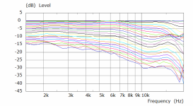
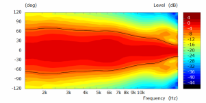
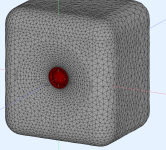
I tried the T34A in a 2-profile geometry, just to see if I'll be lucky on the first try.
It could be optimized further I guess to fix that narrowing around 13k, but I'm really not willing to do that now...


It could be optimized further I guess to fix that narrowing around 13k, but I'm really not willing to do that now...
Code:
HornGeometry = 2

Throat.Diameter = 38
Throat.Angle = 40
Length = 20

Horn.Adapter = {
  L = 5
  k = 0.7
  Width = 50
  Height = 50
  Segments = 6
  ZCtrl = 0.5,0.3,0.5,0.3
}

Horn.Part:1 = {
  L = 15
  Segments = 10
  H = {
  r0 = 19
  a0 = 60
  k = 2
  a = 70
  s = 1.27
  n = 2.15
  q = 0.996
  }
  V = {
  r0 = 19
  a0 = 60
  k = 2
  a = 70
  s = 1.27
  n = 2.15
  q = 0.996
  }
}

Source.Contours = {
  dome WG0 34 10.515 2 1 5 2
}

Source.Velocity = 2   ; axial motion

Mesh.ZMapPoints = 0.3,0.2,0.7,0.9
Mesh.ZMapElementSize = 0.1,0.3,0.25,0.85

Mesh.Enclosure = {
  Spacing = 40,50,40,200
  Depth = 200
  EdgeRadius = 35 ; 25
  EdgeType = 1
  FrontResolution = 8,8,12,12
  BackResolution = 16,16,16,16
}

Mesh.Quadrants = 1        ; =14 for 1/2 symmetry

Mesh.AngularSegments = 64
Mesh.LengthSegments = 16
Mesh.SubdomainSlices =

Mesh.ThroatResolution = 4
Mesh.MouthResolution = 6
Mesh.InterfaceResolution = 6
Mesh.RearResolution = 16

ABEC.SimType = 2
ABEC.f1 = 1500   ; [Hz]
ABEC.f2 = 20000  ; [Hz]
ABEC.NumFrequencies = 40
ABEC.MeshFrequency = 1000   ; [Hz]

ABEC.Polars:SPL = {
  MapAngleRange = -120,120,49
  Distance = 1      ; [m]
  NormAngle = 0
}

Report = {
  Title = "ATH-DOME/T34A"
  NormAngle = 10
  Width = 1400
  Height = 900
}

Output.STL = 0
Output.ABECProject = 1Of course you have all the freedom you want, I've never claimed that the shape is any special 🙂On the one hand the R-OSSE has proven to be very helpfull in designing waveguides, on the other hand I feel we don't have to use it, but have more freedom in the shape
Helpful it definitely is, it changes the curvature smoothy all along the curve - it terminates an OS in a very smooth manner. That's all it does.
Last edited:
The shape is special in that it allows for an exact solution along with insights into HOM and their effects. Other shapes will be "OK" but the insight of HOMs will be missing as the direct solution does not separate out the results into "modes" of propagation. To do that one would have to assemble a large matrix and find the eigenvalues and eigenmodes (all of which are complex arithmetic) and that is not a trivial task.There is (at least...) one other thing that not clear to me. The OS was one of the shapes in Gedlee's book where the wave equation could be solved. Does that make the shape special in itself, or is it just one of the few we have a analytic solution for and as such has provided quite some insight courtesy of Gedlee? Are other shapes also just as 'ok' when we have ABEC to do the heavy lifting and provide a numerical solution?
Can it be proven that OS is optimal in any acoustic sense? Probably not, (although it very well might be true.) It does appear that the "best" of the ATH designs look very much like OS merged with an smooth termination, so it's clearly not far from the ideal. The "ideal" shape might be different for a terminated waveguide as opposed to the theoretically infinite OS.
Analytical solutions have their advantages and disadvantages. Simplify assumptions (like an infinite waveguide) make the results less than ideal, but they can give significant insights into what is going on and how to control things like directivity.
Which is what I have been saying is what we want to do.Helpful it definitely is, it changes the curvature smoothy all along the curve
Hi @mabatI tried the T34A in a 2-profile geometry, just to see if I'll be lucky on the first try.
It could be optimized further I guess to fix that narrowing around 13k, but I'm really not willing to do that now...
View attachment 1178003View attachment 1178006
View attachment 1178004View attachment 1178005
As I try to learn ATH + ABEC, I've been trying to run the same scripts others are posting and testing to see if I get similar results, and I couldn't in the case above:
Any idea why that may be the case?
Steps were:
1) Run ATH script above
2) Open Model in AKABAK
3) Start BE Solver
4) Open VACS
5) Back to AKABAK to Calculate All Spectrum Observations.
That is all I did.
Also (for @mabat or @fluid) - can you please share how:
1) to generate polar in line-chart format - is that also VACS?
2) to enable the view included in posts 12,474 and 12,480 in ABEC/AKABAK
3) To measure/calculate tweeter dome geometry: Are you measuring the actual tweeter dome geometry manually, with the physical driver in hand? or are you reaching out to manufacturers for dome geometry specifications? If it's the former, I'm happy to start measuring and sharing based on the drivers I have on hand.
4) When I simulate the waveguide with an enclosure, the calculation takes a bit of time (30 mins in the example above). In post 12,503, an approach was shared to accelerate processing time, and it works. Just curious: it seems the most challenging part to get right is say 7khz and above (i.e. at frequencies where the radiating sound leaves the waveguide before we even make it to the enclosure surface) - Would you say the best approach is first to simulate using the approach included in post 12,503 (I suppose it won't work for non-axisymmetric guides), and get the 7khz+above right first, and then move on to adding/simulating the enclosure?
I'm not completey sure of the reason but I ran into the same issue recently. My hack solution to it was to paste a random static.txt file into the results directory and then it would produce a report 🙂What could be going on here?
Maybe the data in static.txt needs to be accurate but most of it seems to be information.
Attachments
There are some differences in the way observations are handled between ABEC and Akabak, my advice would be to use ABEC with Ath as it is just easier. mabat has a link on his website to the ABEC download if you don't have it. You don't need a full version running in demo mode will still solve and if you have a full version of VACS you can save the spectrum file from there.Any idea why that may be the case?
Possibly you are seeing normalization changes too. Normalized to 10 degrees y value usually looks better and more even. Any changes to ranges or displayed value options can make a difference too.
What I get for the code above
For polar curves as I call them you click on the polar plot and choose curves to contour from one of the menu items.Also (for @mabat or @fluid) - can you please share how:
1) to generate polar in line-chart format - is that also VACS?
2) to enable the view included in posts 12,474 and 12,480 in ABEC/AKABAK
3) To measure/calculate tweeter dome geometry: Are you measuring the actual tweeter dome geometry manually, with the physical driver in hand? or are you reaching out to manufacturers for dome geometry specifications? If it's the former, I'm happy to start measuring and sharing based on the drivers I have on hand.
4) When I simulate the waveguide with an enclosure, the calculation takes a bit of time (30 mins in the example above). In post 12,503, an approach was shared to accelerate processing time, and it works. Just curious: it seems the most challenging part to get right is say 7khz and above (i.e. at frequencies where the radiating sound leaves the waveguide before we even make it to the enclosure surface) - Would you say the best approach is first to simulate using the approach included in post 12,503 (I suppose it won't work for non-axisymmetric guides), and get the 7khz+above right first, and then move on to adding/simulating the enclosure?
Fields are what you need to set up for the views in that post and are solved separately.
I have used both, Bliesma came from the manufacturer, SB from augerpro's physical measurements.
It took my laptop 23 mins so 30 is not bad. Circsym will slove much quicker particularly to higher frequencies. I wouldn't get carried away with trying to make anything above 10K 'perfect' as the liklihood that reality will match is starting to get small. Above 10K so much can change. You will save a lot of time by solving to 10 or 15K first with a coarser mesh. In the super wide dome waveguides the encosure adds a lot of computation time but it is important if you want a relatively accurate answer.
I'm not completey sure of the reason but I ran into the same issue recently. My hack solution to it was to paste a random static.txt file into the results directory and then it would produce a report 🙂
Maybe the data in static.txt needs to be accurate but most of it seems to be information.
Thank you, Fluid! This did the trick.
- Home
- Loudspeakers
- Multi-Way
- Acoustic Horn Design – The Easy Way (Ath4)