Acoustic Horn Design – The Easy Way (Ath4)

[fluid]

Ha Ha yes, "trivial" can be used in a negative way. I took no offence. Unfortunately I still don't understand it yet. I will try and work it out later. Honestly I don't mind if you explain it to me like I'm a five year old

 

[mabat]

What we do here is using one period of the sine function, i.e. for angles 0 - 360 deg, which is also the angle around the waveguide axis. The parameters set the particular values between which the function oscilates:

Desmos - angular function in cartesian coordinates

 

[mabat]

Here you can see the angle values better:

Ath angular function (1)
Ath angular function (2)
Ath angular function (polar)

 

[fluid]

OK I think I get it now how the values in the example were arrived at. You either use a + or - to get the difference between the horizontal or vertical values in the non blended curves and use that as a number before *sin(p)^2.

 

[mabat]

Yes. The sign simply depends on what is bigger, 'h' or 'v'. The formula automatically accounts for that.

value_at_p = h + (v - h)*sin(a*p)^n

 

[limacon]

Iteration 39 wip. Thanks mabat for a wonderful tool. Looking forward to measuring this one. Will start a new build thread. Hmm. What to call it...?

 

[limacon]

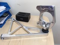
Mindsource. Chisel? No. Just haste. OT - spending more time on my new EV car bits.

 

[jzagaja]

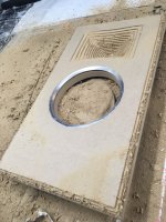
Iteration 39 wip. Thanks mabat for a wonderful tool. Looking forward to measuring this one. Will start a new build thread. Hmm. What to call it...?

Quite deep rough machining

 

[limacon]

Getting my head around exponential shapes on the real wall of the cabinet. A fairly shallow Hyp-Exp shape followed by a shallow Hyp-Exp rear port flare. Yields interesting spl curve with low port noise and less box resonance. 12p80nd with -f3 ~ 85Hz. A la "LineSource" again. Port air velocoty sub 1ms-1. Now to figure out exp driven curves in Solidworks...

 

[mabat]

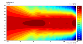
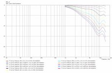
I have finally managed to finish the circular symmetry output. Sample simulation of a free-standing demo waveguide: 100 frequency points, 500 Hz - 20 kHz, mesh frequency 40 kHz. Solving time: 11 seconds

Probably available in 4.6.2 some day...

 

[mabat]

200 frequency points, 60 kHz mesh frequency: 57 seconds

 

[mabat]

Linear frequency abscissa...
I think that for an axisymmetric waveguide development we can't wish more.

 

[Patrick Bateman]

What type of system are you using?

My desktop is a dual xeon with sixteen cores, but it's probably about time to replace it, because the single core performance is so poor (just 2ghz per core.)

My laptop is an Ryzen quad core, and takes about 30 minutes to solve my Abec sims.

 

[mabat]

No, the trick here is the axial symmetry - ABEC/AKABAK has a special computation mode for that. So this is not a full 3D simulation, it is only applicable to axisymmetric devices. In that case it is possible to reduce the calculations considerably.

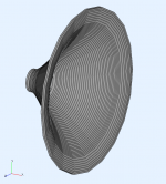
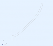
This is the whole "mesh" in this particular example:

 

[mabat]

For me this is about the only way how to reasonably simulate and optimize big axisymmetric waveguides I would like to make. With full 3D sims it would take eternity...
Now I can easily test 10+ iterations in a hour.

 

[orreborre]

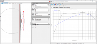
I've done an attempt at copying the Visaton WG148R to have some kind of benchmark design to compare my designs with. I traced the profile from the drawing and matched it in ath:



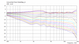
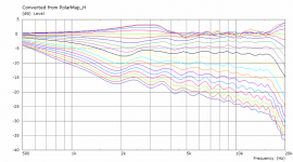
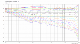
It simulates like this:


Comparing the simulation with the measurements at Test Seas Noferro-900 Visaton Waveguide WG-148R we see that the measurement has a better directivity control at lower frequencies, which I guess is because it is measured in an finite baffle. So, does anyone have a nice method to add an baffle to an ath produced waveguide and simulate it like that instead? It would be nice to compare the results

Here are the ath parameters for those interested:
Geometry.Definition = 1
Throat.Profile = 1
Throat.Diameter = 38
Throat.Angle = 15
Coverage.Angle = 40
Length = 21
Term.s = 2.25
Term.n = 2.25
Term.q = 0.999

 

[mabat]

Adding a finite baffle/enclosure is in the pipeline.

 

[jcarothers]

mabat - what is the purpose of the mesh on the rear side of the horn (to the left of the main waveguide profile) in your image? I've been experimenting with CircSym as well, but with only the inner profile and an IB.

 

[mabat]

By rotating around the X axis this makes a free standing horn. There's no IB in this case (it is still a possible option, of course), here I'm interested in free standing waveguides - big ones.

 

[jcarothers]

Got it! Makes sense why there appear to be some ripples/diffraction from the edge in that case. I've done similar simulations with circsym and a dome tweeter profile and they appear much smoother due to the infinite baffle.