Each source model applies to any system that is emulating or behaving like it.O.k., got it, but does this apply to any of both systems
The ESL-63 theoretical starting point was to emulate the portion of the wave-front coming from a point source or pulsating sphere that would pass thru the diaphragm if it was placed 30cm behind diaphragm. The FrontRo theoretical starting point was to emulate the motion of the outer surface of an oscillating sphere. Both speakers use rings and delays, but the acoustic source that they behave like is different.
One way to think about how the ESL63 emulates a portion of the wave-front from a pulsating sphere is to consider the ESL as acoustically transparent, like an open window. So, place a window the size of the ESL63 in an otherwise acoustically inert, infinitely sized wall. Now place a point source, or pulsating sphere source 30cm on the back side of the wall centered on the window, and you listen from the other side sitting your usual listening distance from the window. Next, stretch a very thin diaphragm across the window. Other than a very small roll off in the highs from the diaphragm mass(which can be compensated for) you would not notice any difference compared to the open window. Now, calculate the relative pressure and time delay across the window at the plain of the diaphragm. Knowing this, you could add stator rings and drive signal to move the diaphragm to re-create this same pressure field vs time across the whole window. Finally, remove the source behind the wall and turn on the power to the ESL.Seeing the ESL63 as an pulsating sphere is not the first thing that comes to my mind.
Summing up currents for all the segments in your model and you get the Fig. 14 response from the AES paper. Nicely done 🙂Here is an initial LTSpice model that I have made for the FrontRo ESL.
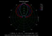
For grins, I took the currents from you model and applied them to rings to calculate the polar response.
Attachment #1: This is the traditional polar plot which matches Figure 13 from the AES paper.
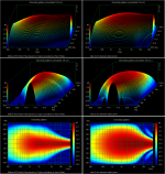
Attachment #2: The polar response for the Hans’ FrontRo model is shown in the 3 plots on the left side.
For comparison, the polar response for an ideal 2 inch diameter piston is shown on the right side.
Attachment #3: Because I know somebody would ask 😉 The polar response for the first 6 rings of Hans’ ESL-63 model is shown in the 3 plots on the left side. For comparison, the polar response for just the center disk of the ESL-63 is shown on the right side. This basically tells us that the directivity of the whole ring system at high frequency is not that much different from that of just the inner disk, but it can play 15dB louder.
Attachments

Each source model applies to any system that is emulating or behaving like it.
The ESL-63 theoretical starting point was to emulate the portion of the wave-front coming from a point source or pulsating sphere that would pass thru the diaphragm if it was placed 30cm behind diaphragm. The FrontRo theoretical starting point was to emulate the motion of the outer surface of an oscillating sphere. Both speakers use rings and delays, but the acoustic source that they behave like is different.
One way to think about how the ESL63 emulates a portion of the wave-front from a pulsating sphere is to consider the ESL as acoustically transparent, like an open window. So, place a window the size of the ESL63 in an otherwise acoustically inert, infinitely sized wall. Now place a point source, or pulsating sphere source 30cm on the back side of the wall centered on the window, and you listen from the other side sitting your usual listening distance from the window. Next, stretch a very thin diaphragm across the window. Other than a very small roll off in the highs from the diaphragm mass(which can be compensated for) you would not notice any difference compared to the open window. Now, calculate the relative pressure and time delay across the window at the plain of the diaphragm. Knowing this, you could add stator rings and drive signal to move the diaphragm to re-create this same pressure field vs time across the whole window. Finally, remove the source behind the wall and turn on the power to the ESL.
Cogent & elegant description!
Imagine this speaker been developed in the 60-70ties.
Walker did some speaches at AES and got standing ovations.
Wish i had been there..
Walker did some speaches at AES and got standing ovations.
Wish i had been there..
With Steve Bolser's and Demian's fantastic support, I could bring my LTSpice model to an end.
After having added all currents, currents that are directly proportional to the produced SPL, I added all the necessary acoustic corrections.
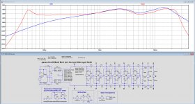
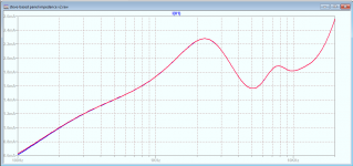
First image below shows in blue the sum of all currents and the red curve shows the end result after having applied the various corrections, such as:
Membrane resonance at 50Hz, Proximity effect a 1 m distance, Baffle effect and stator transparency.
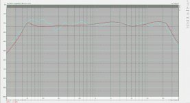
Second image shows an acoustic recording with om the top the final result from LTSpice.
Be aware that all this applies only to the on axis response.
Hans
After having added all currents, currents that are directly proportional to the produced SPL, I added all the necessary acoustic corrections.
First image below shows in blue the sum of all currents and the red curve shows the end result after having applied the various corrections, such as:
Membrane resonance at 50Hz, Proximity effect a 1 m distance, Baffle effect and stator transparency.
Second image shows an acoustic recording with om the top the final result from LTSpice.
Be aware that all this applies only to the on axis response.
Hans
Attachments
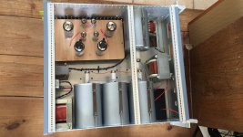
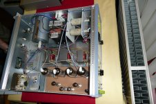
I wanted to know the actual panel current which would have to be provided by a direct drive amp, so I decided to try to measure it on one of my spare ESLs.
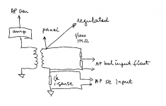
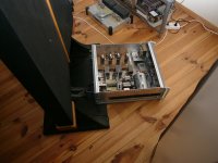
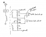
The first attachment shows the test setup. I drive the speaker (one channel) from the AP generator, through a power amp. I feed a sample of the hv transformer output to one channel of the AP and use the 'regulate' option to make sure that the xformer output voltage remains constant with frequency, here I regulate to 250V.
I have a 1k current sense resistor in the ground leg of the secondary and measure the voltage representing xformer current into the panel.
The 2nd attachment shows the measured current, and the 3rd shows the current as 'measured' by the simulation of the latest panel model as the 4th attachment. What you see is a large discrepancy between measurement and simulation. So first question: is my measurement setup kosher?
Jan
Attachments


I would regulate on the primary side before the 1,5 (0,75ohm) Ohms resistors.
Maybe 100 ohm shunt instead of 1k.
100 ohm source impedance is closer to the coax that i guess you are feeding to AP?
Maybe 100 ohm shunt instead of 1k.
100 ohm source impedance is closer to the coax that i guess you are feeding to AP?
The simulation is on the panel itself, so regulating on the primary side would no longer make the two situations comparable.
The AP has 100k input R so 1k is OK. 200pF cable C with 1k source has a -3dB freq of > 6MHz.
I did think about this .... ;-)
Jan
The AP has 100k input R so 1k is OK. 200pF cable C with 1k source has a -3dB freq of > 6MHz.
I did think about this .... ;-)
Jan
Anyone tried a direct drive amp on one of these?
Attachments
Last edited:
In your drawing, you don't specifically show what you have done with the other panel connection. Is it still connected to the output of the other step-up transformer? or have you moved it to ground for the measurement. From your measurement results, I would guess it is still connected to the other output transformer.... is my measurement setup kosher?
Attachments
Ahhh yes! It is still connected, and of course I should do my measurement differential!
Back to the drawing board!
Jan
Back to the drawing board!
Jan
Anyone tried a direct drive amp on one of these?
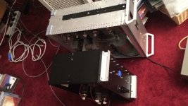
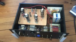
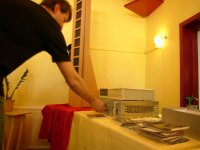
Your amplifier looks familiar to me. Can it be that I saw this several years (many years?) ago at a meeting of the Dutch ESL club?
BTW I am working on a DD amp, hence my measurements/questions.
Jan
Jan- Do you have a current probe?
I can duplicate your measurements with a current probe, but it will be a week or two before I'm able.
I could also just drive a panel from a HV amp and measure the current. I thought I made some measurements but have not found them.
Measuring the drop across a resistor should work but you may have a common mode issue. Easy test- short the resistor and sweep. You should get nothing. Any output is an indication of common mode errors. You are trying to measure millivolts in the presence of 100V. Not easy.
Demian, I have a current probe (Tek TCP312 with amplifier) but it's pretty noisy at these low currents.
I will redo my measurements later today, fully balanced.
Jan
I will redo my measurements later today, fully balanced.
Jan
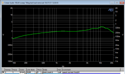
OK, re-done, balanced. There is still a discrepancy between measured and simulated, but it gets closer.
Up to a kHz it is pretty close, but of course we are interested in what lies above.
It's also reasonable close above 5kHz. The big elephant is the bump at 2.2kHz.
Edit: measurement is done with speaker close (<1 ft) to a wall. I redid the measurement moving it further away (3ft), no change.
Comments?
Jan
Attachments
Last edited:
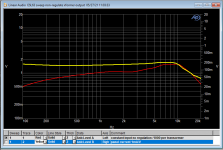
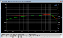
The plot thickens. This is the same measurement, but now with the panel voltage not regulated, i.e. constant level input to the speaker input, so the measurement now includes the effect of the input crossover filter & transformer. The 1.5R//220u has a xover of around 500Hz, and then there's also the xformer non-flat response I guess.
RED is the voltage on the panel, with constant input voltage to the speaker. There is a dip exactly at the peak that is shown in the simulated panel current.
Also, above 10kHz the panel voltage drops, with the result that the measured panel current is much lower than in the simulated panel current with constant panel voltage.
I believe that in the case of direct drive, the drive voltage should be equalized according to the RED curve, which then also significantly lowers the maximum drive current requirement.
Am I right?
Jan
Attachments
Last edited:
Yes, i have demoe'd one set long time ago (2007) at the ESL club.
Attachments

Last edited:
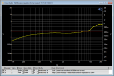
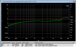
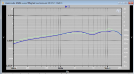
My face is red - I made a hook-up mistake, so the previous graphs are incorrect. Here the correct ones - but not significantly different.
First one is with panel voltage regulated to 250V per panel (500V total).
Second is without regulation, constant input to the amp, and panel voltage varies due to xover and xformer non-linear response.
Third is as the 2nd but with the 1Meg measurement load across the panels removed. The panel current is a bit higher, as expected due to higher panel voltage, but exact panel voltage not known.
Fourth is again the test setup.
Sorry for the confusion, I think I've got it right now.
Jan
Attachments

- Home
- Loudspeakers
- Planars & Exotics
- QUAD 63 (and later) Delay Line Inductors