Can the reference error be quantified in terms of Gm error or Hfe error? Errors from random noise may cause limitations to THD extrapolations.
An IC buffer would be easier to solder, the advantage of discrete would be higher rails and higher current but your design doesn't take advantage of the higher voltage or have much need of it. So I guess the question is what transistors would suffer from a lower base drive limit?
An IC buffer would be easier to solder, the advantage of discrete would be higher rails and higher current but your design doesn't take advantage of the higher voltage or have much need of it. So I guess the question is what transistors would suffer from a lower base drive limit?
The DAC, DAC8563, is 16-bit, 4LSB INL with internal 2.5V Ref In/Out. Its bidirectional Ref has +-5mV (0.2%~0.4% for 2.5V) initial Accuracy and 10ppm temp drift, 12uVpp 0.1-10Hz noise.Can the reference error be quantified in terms of Gm error or Hfe error? Errors from random noise may cause limitations to THD extrapolations.
An IC buffer would be easier to solder, the advantage of discrete would be higher rails and higher current but your design doesn't take advantage of the higher voltage or have much need of it. So I guess the question is what transistors would suffer from a lower base drive limit?
I don't know how to calculate the error propagation, but since this voltage reference also supply to ADC as Vref, I think it's better to have independent Vrefs, at least this avoids DAC-ADC thermally dependent as they share one common Vref.
The IC buffer I proposed is BUF634, which has the ability to sink/source 250mA, I guess that's enough for most cases? For some TO-92 BJTs, down to ~10uA Ib is required. The reason I want to use (maybe) IC is that it saves lots of time for soldering and debugging, especially if the PCB is soldered by users, discrete design might need efforts to debug.
So is the VC channel, the VC requires high power output ability, and power OPamp like OPA541, OPA549 even Apex PA04 come into my mind. OPA541 might be better, as it's rated +-40V supply, 10A peak output; it provides 5A continuous output between ±(|VS|– 4.5). Hence, if it's supply with ±40V, OPA541 can almost meet the requirement of the design, ±36V& Io>5A.
After discussion with the author, we reached a consensus that use the Arduino Nano as the microprocessor instead of discrete ATMEGA328P.
This saves time for soldering and debugging of ATMEGA328P, including USB-Serial converter, either FT232 or CH340.
The Arduino Nano integrates Atmega328P and USB-Serial converter, also the Vin to +5V conversion.
So, the user can simply plug a Nano into the socket, use the USB port to update the firmware and receive/send data from the device.
Hi,Can you plot early voltage vs Vce?
After writing the manual, there's a part that talks about Early effect.
Although the iTracer program cannot plot a graph of Early Voltage vs Vce,
but the Early Voltage, or the Early effect is actually taken into consideration of tracer's processing algorithm.
The software uses lots of mathematical models to describe and compare transistors, which makes transistor matching more precisely and quickly.
The Manual is on the way, and it explain how this tracer deal with "describing" transistors and matching, managing them.
Maybe the most different and innovative feature of this tracer is that massive mathematical proceesing is used in the development of the tracer's core.
I was curious because it actually takes a lot of resolution to plot that curve accurately without noise, and I have been looking for something that can do it. If your hardware is good I can just work the curves in a spreadsheet.
Early Voltage vs. Ibase is more illuminating IMHO.
Fit a quadratic or cubic spline to the (noisy) measured data at Ic >> Iknee, then extract Vearly from the fitted spline
Fit a quadratic or cubic spline to the (noisy) measured data at Ic >> Iknee, then extract Vearly from the fitted spline
Yes, we actually did that.Early Voltage vs. Ibase is more illuminating IMHO.
Fit a quadratic or cubic spline to the (noisy) measured data at Ic >> Iknee, then extract Vearly from the fitted spline
The program uses fitting functions and weighting to process curves, some of the coefficients of the fitting function are used to calculate or parameterized transistors, thereby making matching transistors possible and reasonable.
The Manual will talk more about math details, and it is kind of huge work so I am stilling working with.
I was curious because it actually takes a lot of resolution to plot that curve accurately without noise, and I have been looking for something that can do it. If your hardware is good I can just work the curves in a spreadsheet.
After discussion, the author agreed for 5 MCUs for free sampling, there are pre-programed Arduino Nano.
Also, I am making layout of the PCB, my plan is to make 5 fully-assembled tracers for sampling.
Anyway, there are 5 programed Arduino NANO here, and the schematic is open for EasyEDA and Altium.
If you are interested and able to layout, maybe I can send you a MCU?
About the hardware, DAC8562 and ADS1115 are used.
DAC8562 is a 16-bit DAC, with INL 4LSB.
ADS1115 is a 16-bit ADC, with INL 1LSB.
A spline? That will not work to extrapolate to Vearly.Early Voltage vs. Ibase is more illuminating IMHO.
Fit a quadratic or cubic spline to the (noisy) measured data at Ic >> Iknee, then extract Vearly from the fitted spline
You might try a polynomial (1st, 2nd or 3rd) to extrapolate, but the uncertainty in the extrapolated result will be huge.
"extract" isn't the same thing as "extrapolate".
"extract Vearly" means "perform a linear regression, and interpret the X-intercept of the fitted line as the best estimate of (-Vearly)" since the X-intercept will be a negative number (for NPN) but Vearly is positive by convention.
The purpose of the fitted spline step is to reduce noise in the raw measurement data. Then linear regression is performed after noise reduction.
Ok, that makes a bit more sense. However, I still don't see how you intend to use the spline. Splines are typically used to draw smooth lines between data points. They don't reduce the noise in the data points. Also, there's no magic way to remove the uncertainty due to (random) noise in the raw data. The only way to improve this is by better (less noisy) data.
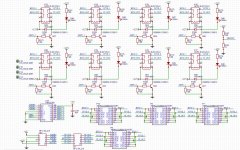
The lastest revision of the iTracer, and Altium Sch files are attached, any suggestions are welcomed.
People can make their own iteration of PCB based on the Altium files, or you can wait for my iteration that will be published later.

People can make their own iteration of PCB based on the Altium files, or you can wait for my iteration that will be published later.
Attachments
If you have a LOT of datapoints, laying the spline to some kind of average will average-out the scatter.Splines are typically used to draw smooth lines between data points. They don't reduce the noise in the data points.
What kind of average? is a real question. mean? RMS? min+max/2?
No, the splines will not reduce the noise. The averaging applied to the data BEFORE calculating the spline will.If you have a LOT of datapoints, laying the spline to some kind of average will average-out the scatter.
The choice of the averaging function should depend on the type of noise. For example, if the noise follows a normal distribution, a good old mean may be good. If outliers are a problem, the median function is useful.
Last edited:
If you have a LOT of datapoints, as PRR posits, then
Fitting a cubic function (4 degrees of freedom, i.e., 4 coefficients) to (N >> 4) datapoints, averages out some noise. The greater the N, the greater the noise reduction. Doing this to overlapping segments of the raw input data, produces a smooth(er) curve. The second step, (fitting a linear function a/k/a linear regression) upon that smoother curve, gives an X-intercept which represents an improved estimate of -Vearly.
A quadratic function (3 coeffs ---> 3 degrees of freedom) gives a slightly different tradeoff of noise reduction vs. fitting error vs. number of overlapping segments.
Last edited:

Take a look at Savitzky-Golay Filters: https://en.wikipedia.org/wiki/Savitzky–Golay_filterIf you have a LOT of datapoints, as PRR posits, then
Fitting a cubic function (4 degrees of freedom, i.e., 4 coefficients) to (N >> 4) datapoints, averages out some noise. The greater the N, the greater the noise reduction. Doing this to overlapping segments of the raw input data, produces a smooth(er) curve. The second step, (fitting a linear function a/k/a linear regression) upon that smoother curve, gives an X-intercept which represents an improved estimate of -Vearly.
A quadratic function (3 coeffs ---> 3 degrees of freedom) gives a slightly different tradeoff of noise reduction vs. fitting error vs. number of overlapping segments.
However, no matter what you do, the noise in the raw data will always limit the uncertainty of the Vearly value. There is just no magic trick to remove the uncertainties of derived parameter values due to noise in the raw data. The only way out is to get better raw data with less noise.
Well, looking at the plot in post #30, it is not so much "noise" (these are 140dB parts) as simple lack of data (I posited wrong). In the low Vce area there's only 4 or 5 points. Is that typical, hard-coded, or user-set? Can we get some more points in there? In SPICE I would plot this area with 10mV steps.takes a lot of resolution to plot that curve accurately without noise
True. It looks like these measurements were done at a Vc resolution of about 1 V, and one might prefer a somewhat better resolution to get smoother curves at low Vc values. However, higher Vc resolution would not change much in the saturation region, so the extrapolation of the curves from the saturation region to to Ic = 0 to get Vearly will come out pretty much the same.Well, looking at the plot in post #30, it is not so much "noise"
What is the resolution limit of the hardware?
Thank you, this is very close to how the software deal with Vearly. There are some discussion in the manual that talk about this.If you have a LOT of datapoints, as PRR posits, then
Fitting a cubic function (4 degrees of freedom, i.e., 4 coefficients) to (N >> 4) datapoints, averages out some noise. The greater the N, the greater the noise reduction. Doing this to overlapping segments of the raw input data, produces a smooth(er) curve. The second step, (fitting a linear function a/k/a linear regression) upon that smoother curve, gives an X-intercept which represents an improved estimate of -Vearly.
A quadratic function (3 coeffs ---> 3 degrees of freedom) gives a slightly different tradeoff of noise reduction vs. fitting error vs. number of overlapping segments.
(Forgive me that I am not the EE, and the following is just my translation of the manual that the author send me)
The output function of BJT could usually defined by:
Ic=A−Ke^(−Buce)|Ib
This fitting function indicates that Ic is the function in terms of uce given Ib, where A, K, B are the constants that describes the characteristic curves.
However, if one seriously looks at the formula, problems could be found.
Now, imagine if Uce is very large, the second term in the formula Ke^(-Buce) is nearly 0;
this makes Ic=A, the curve becomes horizontal line which is not the real case.
In reality, because of Early effect of transistors, tangents to the characteristics at large voltages extrapolate backward to intercept the voltage axis at a voltage called the Early voltage, often denoted by the symbol VA:
Apparently, the BJT output function must be modified to reveal the reality:
Ic=A−Ke^ (−Buce)+K1uce|Ib
K1uce is added, where K1 stands for the slope.
Finally, we have 4 coefficients A, K, B, K1 in the formula.
Take a closer look, one can realize that A reflects the Ic in the turning (Knee) point between saturated(non-linear) and non-saturated(linear) area.
So, clearly A is a very important constant of the function.
Coefficients K, B describe the curvature from non-linear to linear area;
in most cases, K and B are not as important as A.
K1 defines the slope of linear area of the curve, which determines the similarity of different curves.
All these coefficients influence the curve’s shape by different extent.
----------------------------------------------------------------------------------------------------
- Home
- Design & Build
- Equipment & Tools
- New Tracer is coming