I had noticed the same/similar change in bass response vs listening distance but hadn't attributed it to the U-frame flattening out. In fact, the abec generated responses don't show this when I compute response at 6m instead of the usual 3m but it appears I should look at 1.5m instead of 6m. Nevertheless, it or something like it shows up in the system simulation, where in these plots, the U-frame plays down to 50 Hz.

My usage model is with the speakers toed in at each end of my desk, resulting in a 1.5m listening distance for background music while I work. Then I can push back to 3m for foreground music or TV. I had planned two EQ presets to deal with this.
My usage model is with the speakers toed in at each end of my desk, resulting in a 1.5m listening distance for background music while I work. Then I can push back to 3m for foreground music or TV. I had planned two EQ presets to deal with this.

the resonances of concern are front to back, not side to side...One question- with u -frames the quarter freq is noted as a concern due to resonances. Doesn't this issue become less of a concern if the walls of the u-frame are not parallel? That is, if the u-frame flares towards the rear with non-parallel sides, resonances do not form at the usual 1/4 wavelength?
I wanted to present the U-frame response in full detail so here goes. I'm just going to attach the files.
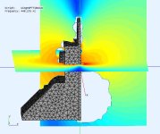
The U-frame is a modest 118 mm deep. It sits above a sealed sub mounted on the rear facing slanted baffle you can see in the fields diagram.
The U-frame is a modest 118 mm deep. It sits above a sealed sub mounted on the rear facing slanted baffle you can see in the fields diagram.
Attachments
-
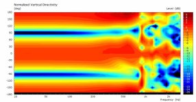 wingPTT10_PolarMap_V_norm.jpg36 KB · Views: 99
 -
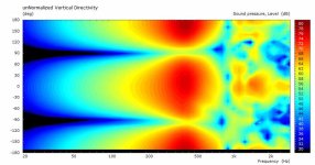 wingPTT10_PolarMap_V_nonorm.jpg34.3 KB · Views: 82
 -
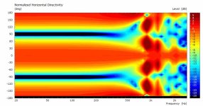 wingPTT10_PolarMap_H_norm.jpg36.2 KB · Views: 89
 -
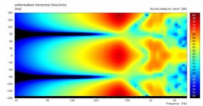 wingPTT10_PolarMap_H_nonorm.jpg34.1 KB · Views: 85
 -
 wingPTT10_Curves_V_norm.jpg56.7 KB · Views: 86
 -
 wingPTT10_Curves_V_nonorm.jpg53.4 KB · Views: 91
 -
 wingPTT10_Curves_H_norm.jpg43.3 KB · Views: 95
 -
 wingPTT10_Curves_H_nonorm.jpg43.3 KB · Views: 101
 -
 fields_440_wings.jpg39.2 KB · Views: 106
I'll also show the simulation files as they may also be of interest.
One starts with a sketch of what is to be modeled and labels each vertice with an ID and its coordinates in 3D space.
Then sketch is then converted to a list of "Nodes" in ABEC parlance.
As part of this conversion, the coordinates are parameterized in an ABEC "Formula" list to facilitate modelling different size structures.
The result is the attached Nodes.txt.
This file didn't start out so complex. It started with just the baffle and then evolved into what you see. My sketches, although derived from my Sketchup files are too ugly to share.
Attachments
Next is Elements.txt where vertices are connected to form surfaces.
In the file, you will find "Baffle" statement for the front and rear of the baffle. At the end of each block, you list the vertices of the baffle, allowing arbitrary shapes to be created. The driver(s) can be positioned anywhere on the baffle.
There are also "Element" statements for other structures such as the sides/edges of the baffle and the subwoofer cabinet. The order in which you list the nodes of a surface affects which way the "normals" point, which is another way of saying whether the surface is an inside or an outside. You should always check the normals since they must be correct for an accurate simulation.
The "Duct" statement creates a hole through the baffle, which is critical and needs finer meshing to avoid gaps in the mesh between it and the baffle surface.
Finally, you have diaphragm statements, for both front and rear of the driver if modelling a dipole/U-frame, and also for a vented cabinet.
The diaphragm model includes a number of parameters that allow modelling the gross characteristics of the cone and magnet structures. Parameter values can be found in or deduced from the driver's data sheet. There is a little bit of guesswork in this if you don't have hands on a driver for measuring directly.
Attachments
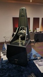
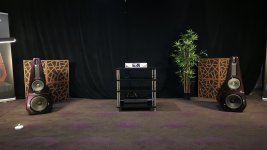
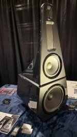
@adason found this at the Capitol Audiofest.
Its a relative of what I have on the drawing board. Sealed sub at bottom. Uframe mid but planar dipole top end instead of coax.
He didn't say who makes it; I imagine its quite expensive...
Its a relative of what I have on the drawing board. Sealed sub at bottom. Uframe mid but planar dipole top end instead of coax.
He didn't say who makes it; I imagine its quite expensive...
Attachments
If the top and sides are flared or top open, wouldn't this be a non issue then? Aren't you concerned about resonances in a closed air column? If it isn't closed, how can there be any resonance?the resonances of concern are front to back, not side to side...
Last edited:
I heard if few times, very nice sound, yes. Great concept.@adason found this at the Capitol Audiofest.
Its a relative of what I have on the drawing board. Sealed sub at bottom. Uframe mid but planar dipole top end instead of coax.
He didn't say who makes it; I imagine its quite expensive...
Attachments

I'd better keep going - that Consonus speaker (above post) sells for around $80K! This is looking like a $10K project for me including amps, DSP, wood and woodwork
I've had my head down in ABEC simulations for the last month. I took a morning off from my own design to develop a model for the Bitches Brew U-frame, which was its inspiration. I think its worth sharing this, given the high amount of interest around Live Edge Dipole family.
Here is the simulation model, drawn by ABEC from a list of points with parameterized dimensions, read off a Sketchup drawing. The model is easily adjusted for height and width of the baffle, the slant of the Uframe wings, and driver type and location.

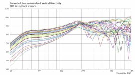
the simulation takes about 18 minutes on my 8 core Ryzen machine and produces this axial SPL. One of the puzzles for me was rationalizing the absolute SPL magnitude against the data sheet sensitivity at 2.83V, 1m. The simulation observes the SPL at 4m distance so I gave it 4V RMS input, instead of 1V RMS, to make up for the -12 db loss for the two doublings of distance. The simulation is in 4pi space so add 6db for the floor. In room, there will be support from the front wall as well below 100 Hz. The data sheet measurement was made on a relatively large IEC baffle, so there is baffle loss to account for as well. The numbers may or may not add up exactly, but the simulation certainly confirms there is enough SPL for the intended use.

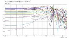
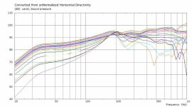
The green trace in the graph is the rear wave. The red is the sum of front and rear and looks useable well past 200 Hz, although the dipole side nulls are gone by then. The deep nulls in the rear wave are, I believe, interactions with the driver magnet structures and the side walls. In other simulations, I've been able to make them disappear by simulating absorption on the sidewalls, or removing the magnet structure from the simulation. With shallow wings in the 50-100mm depth range, these limit the upper operating range of the U-frame. Here, it seems that the dipole range is limited simply by the depth of the wings. They go so far back so very little SPL gets back there to be cancelled, except at very low frequencies. You can see that in how little of the rear wave reaches the front above 200 Hz.
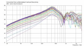
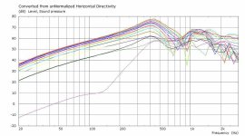
The polar maps and curves extracted from them are attached.
For my own design, I wanted dipole directivity to 400 Hz, so it won't have any wings at all. To make up for the loss of LF, I'll have a shallow mount subwoofer sitting on the floor behind the dipole and facing up. With that, I just need a single dipole mid-woofer.
Here is the simulation model, drawn by ABEC from a list of points with parameterized dimensions, read off a Sketchup drawing. The model is easily adjusted for height and width of the baffle, the slant of the Uframe wings, and driver type and location.
the simulation takes about 18 minutes on my 8 core Ryzen machine and produces this axial SPL. One of the puzzles for me was rationalizing the absolute SPL magnitude against the data sheet sensitivity at 2.83V, 1m. The simulation observes the SPL at 4m distance so I gave it 4V RMS input, instead of 1V RMS, to make up for the -12 db loss for the two doublings of distance. The simulation is in 4pi space so add 6db for the floor. In room, there will be support from the front wall as well below 100 Hz. The data sheet measurement was made on a relatively large IEC baffle, so there is baffle loss to account for as well. The numbers may or may not add up exactly, but the simulation certainly confirms there is enough SPL for the intended use.
The green trace in the graph is the rear wave. The red is the sum of front and rear and looks useable well past 200 Hz, although the dipole side nulls are gone by then. The deep nulls in the rear wave are, I believe, interactions with the driver magnet structures and the side walls. In other simulations, I've been able to make them disappear by simulating absorption on the sidewalls, or removing the magnet structure from the simulation. With shallow wings in the 50-100mm depth range, these limit the upper operating range of the U-frame. Here, it seems that the dipole range is limited simply by the depth of the wings. They go so far back so very little SPL gets back there to be cancelled, except at very low frequencies. You can see that in how little of the rear wave reaches the front above 200 Hz.
The polar maps and curves extracted from them are attached.
For my own design, I wanted dipole directivity to 400 Hz, so it won't have any wings at all. To make up for the loss of LF, I'll have a shallow mount subwoofer sitting on the floor behind the dipole and facing up. With that, I just need a single dipole mid-woofer.
Attachments
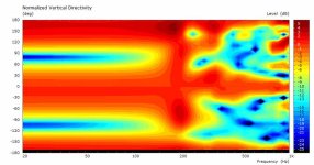
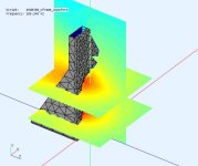
I think the fields diagrams are really interesting, so I'll just attach a bunch of them in order of increasing frequency.
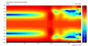
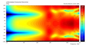
First, fields viewed from above to show H dispersion. These are the fields observed at the level of the upper woofer.


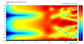
Next we see V fields, viewed from the side:


After looking at fields for a while, I realized I could plot H fields for both woofers in the same drawing. I'm showing the range of frequencies during which the dipole nulls disappear.


Finally, a rear view:

First, fields viewed from above to show H dispersion. These are the fields observed at the level of the upper woofer.
Next we see V fields, viewed from the side:
After looking at fields for a while, I realized I could plot H fields for both woofers in the same drawing. I'm showing the range of frequencies during which the dipole nulls disappear.
Finally, a rear view:
Attachments
I've attached my simulation model for those that want to play with it.
I suppose at some point I should do a tutorial for exporting directivity files to Vituix but for now I just want to post the model.
I'm hoping someone will tweak the model to match their design and take measurements that can be compared with simulation. I would be happy to adjust the model to what was measured and rerun the sim, because there is a learning curve on ABEC even with a working model to start with.
Also, for someone with a 15OB350 at hand to measure, there are a number of physical driver parameters in the "diaphragm" section of the elements file that I only estimated from the data sheet - like depth of cone, dust cap dimensions, etc. If you could share caliper measurements, that would improve simulation accuracy, although its not likely to make a difference in the Uframe passband.
Attachments
Last edited:
Here is the SPL chart for my dipole model. It shows 75 db SPL at 100 Hz, compared to 85 db for the dual-woofer U-frame. That is a 10 db difference but 6 db is due to the U-frame having two woofers versus only 1 for the dipole.

Last edited:
Interesting, if I run my dual woofer model with a single woofer enabled, it predicts 2 db more output at 100 Hz. Here are lower woofer, upper woofer, both woofers, in that order. This is hard to explain. Perhaps lower woofer rear output cancels upper woofer front and vice-versa, but the idea that a single woofer is better than two borders on preposterous. I thought my "LE" script (effectively the XO schematic) would put the two drivers in parallel by virtue of them being in the same drive group but that might not be the case. I need to rewrite the LE script and elements file so each driver is in its own drive group. That should clarify this.
Its things like this that have kept me busy lately.


Its things like this that have kept me busy lately.
The "problem" frequency region for your woofers is not around 100Hz, it's much lower in frequency. I would gladly trade off a 2dB loss at 100Hz for a 6 dB gain at 30 Hz. Based on the responses in your plot, the challenge will be how to deal with the steep rise near 200Hz.
- Home
- Loudspeakers
- Multi-Way
- Dipole and Uframe models and discussion re' Live Edge Dipoles