Yes, I think it's bollocks tooQuite so. And neither do I (approve) -I just don't consider it to be a test,
Facts are facts, and there is no way to argue with them.See the example below for 1 and for 10 elements with the calculation Zo=sqrt(Zopen*Zshort). There is absolutely no difference between the two.
Cascading is a robust proof of the validity of a model, and if it passes it with flying colors, then it has to be right, and I gracefully accept it.
That said, this cable has a transition zone situated at a much higher frequency, >60kHz. The previous examples were around 2.5kHz, and since I didn't see that transition, I assumed the model was wrong.
Performing a similar cascading test on these examples should show a transition zone at ~2.5kHz. With the 100kHz limit, the 60kHz region is not very visible.
There is another unexplained oddity in one of the previous models: the phase doesn't tend towards -45° as it should.
Here is another company that makes cables with flat conductors very close together. They talk about reduced eddy currents. I have heard these cables several times.
Speaker Cables
Speaker Cables
Hans, we are in agreement in all you posted. However, I was not thinking of determining characteristic impedance using the step..... l explain..
In motion control, a step is used to determine how fast a system can settle to the next position. I use it to determine how the cable limits the speed that the load can follow the step.
With a pure 8R, if I step 8 volts, how long does it take the cable to bring that load's current up to 1 ampere. I can use either multi element LCR, or a transmission line, they are equivalent.
In the Dropbox link George provided (I can always count on you) there is a graph showing the settling time for a load given the cable impedance. Note that as the cable z increases, so does the settling time. In that graph, the settling time goes out over 10 uSec for a normal length cable. In fact, if you scanned cable impedance both above and below load Z, you find that there is a minima cusp when line equals load, that minima being the prop delay end to end, roughly 2nSec per foot. Orders of magnitude beyond humans.
Very important is this distinction....my treatment of a cable pair as a specific impedance transmission line is only valid into the low tens of microsecond timeframe. Try to go longer in time and the simplification of sqr(L/C) falls apart as R and G rear their ugly head.
I only speak of timing which is capable of impacting imaging.
Jn
Here is another company that makes cables with flat conductors very close together. They talk about reduced eddy currents. I have heard these cables several times.
Speaker Cables
Wow, I was unaware that twisting conductors causes eddy current resistance.😕
Sigh.
Jn
Don't get me started. Audience have been peddling the notion that their wires are designed for low eddy currents for years.
There are also two relevant albums of JN deposited at the Gallery
Inductance tests - My Photo Gallery
T-line settling - My Photo Gallery
George
Inductance tests - My Photo Gallery
T-line settling - My Photo Gallery
George
BS audio strikes again. There graph of freq response for different cables has no units, db what? Is this nano volts? Useless. There listening tests are the difference signal, ( the voltage across one wire so itss been amplified 100db? ) thats why there so dramatic, again no reference to the signal. The square wave test shows no time scale. All convenient omissions to hide the BS.
And the error signal there recording is the current thru the speaker which should follow the inverse of the speaker impedance, but it dosnt. Why? Have they fudged the results?
Although the simplified model holds much better than I would have expected, a strange quirk remains: the result from this cable is aberrant:
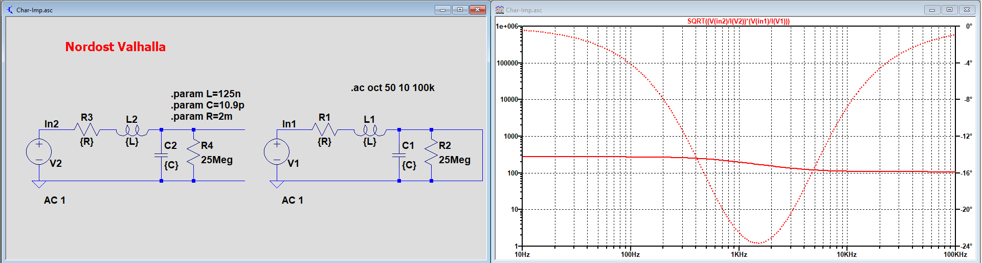
The phase is not right (it should be -45° when F tends to zero), and the magnitude is also too low.
This could mean that hidden parallel conductances have been added somewhere, which is a (lossy) method to keep the impedance flat under the transition frequency.
In my sim, with ideal components, the behaviour sticks to the theory.
The green (1 section) and yellow (12 sections) traces are completely undistinguishable, which is normal if the Zo is correctly extracted from a single cell, and the red trace is a model using a larger lump: all components times 12.
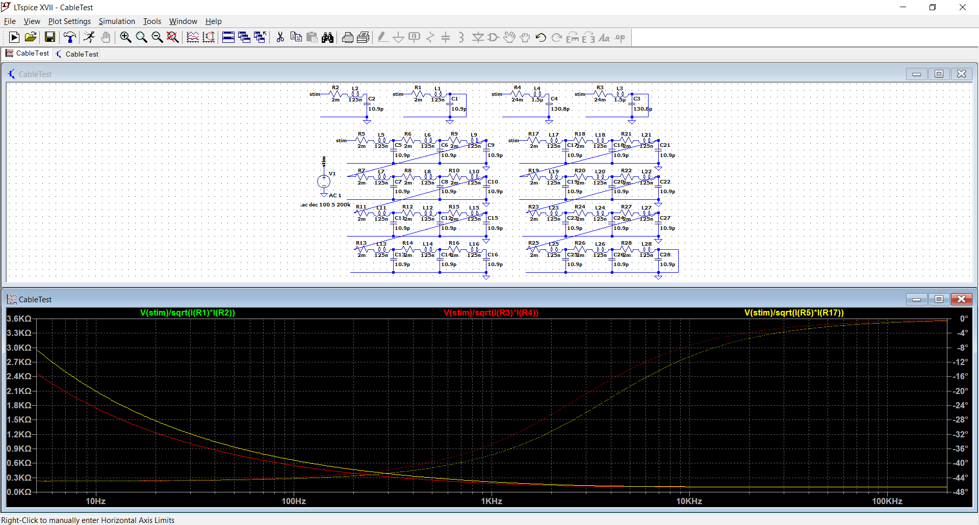
It is slightly different, which is to be expected, but all the curves tend to infinity and -45° when F tends to zero.
The transition around 2.5kHz is also visible.
This is the normal behaviour for a regular TL. If a difference shows, it has to be a hidden parasitic parallel conductance parameter in the elements
The phase is not right (it should be -45° when F tends to zero), and the magnitude is also too low.
This could mean that hidden parallel conductances have been added somewhere, which is a (lossy) method to keep the impedance flat under the transition frequency.
In my sim, with ideal components, the behaviour sticks to the theory.
The green (1 section) and yellow (12 sections) traces are completely undistinguishable, which is normal if the Zo is correctly extracted from a single cell, and the red trace is a model using a larger lump: all components times 12.
It is slightly different, which is to be expected, but all the curves tend to infinity and -45° when F tends to zero.
The transition around 2.5kHz is also visible.
This is the normal behaviour for a regular TL. If a difference shows, it has to be a hidden parasitic parallel conductance parameter in the elements
Attachments

Last edited:
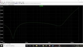
Heres some sims. Used Hans's cable model and a generic speaker model that was handy. The first one is there test, the voltage at the speaker negative. It does not look like there graph and the level is -60db. How did they fudge that? The second is what they should have measured, the error voltage, the voltage difference between the amp and the speaker terminal. As expected the freq variation is less than .05db but the audio they submit has 10db variation. Hard to call it a fudge when its a straight up lie. I feel like posting this in BS auodi comments but Im sure thell erase it instanly.
Attachments


Last edited:
Elvee,
Glad to see that you accepted the Sqrt(open*Shorted) model.
The reason why you have a different phase is because you omitted the 25Meg side to side resistance.
When you add this to your model, you will get the same graph.
Hans
Glad to see that you accepted the Sqrt(open*Shorted) model.
The reason why you have a different phase is because you omitted the 25Meg side to side resistance.
When you add this to your model, you will get the same graph.
Hans
Heres some sims. Used Hans's cable model and a generic speaker model that was handy. The first one is there test, the voltage at the speaker negative. It does not look like there graph and the level is -60db. How did they fudge that? The second is what they should have measured, the error voltage, the voltage difference between the amp and the speaker terminal. As expected the freq variation is less than .05db but the audio they submit has 10db variation. Hard to call it a fudge when its a straight up lie. I feel like posting this in BS auodi comments but Im sure thell erase it instanly.
How does one include the coupling caused by the test loop?
I believe that is what they saw.
Jn
Yup, that's the real identity behind the mask.BS audio strikes again.
I had no problem with the formula per se, I use it frequently myself, I thought that a single RLC cell was too rudimentary to display a consistent behaviour.Elvee,
Glad to see that you accepted the Sqrt(open*Shorted) model.
In general, to simulate or make an artificial line, you need a large number of elementary cells to achieve an acceptable realism, but Zo seems to be an exception.
It is never too late to learn....
Just for the record, here is the mathematical background of the used formula.
When a transmission line with Char. Imp Zo , length L and a with transmission coefficient γ is terminated with an impedance ZL that is different from the Char. Imp. Zo, then at the beginning of the line an impedance Zi will be measured of:
Zi= Zo*(ZL + Zo*tanh(γL))/(Zo+ZL*tanh(γL))
When shorting the line ZL becomes zero and Zi becomes Zshort.
Zshort = Zo*(0 + Zo*tanh(γL))/(Zo+0*tanh(γL)) = Zo* tanh(γL)
When opening the line ZL becomes Infinite and Zi becomes Zopen.
Zopen= Zo*(Inf + Zo*tanh(γL))/(Zo+Inf*tanh(γL)) = Zo*(1+(Zo/Inf)* tanh(γL))/((Zo/Inf) + tanh(γL))
resulting in:
Zopen = Zo/(tanh(γL))
The Char Imp can now simply be calculated as follows:
Sqrt(Zshort*Zopen) = sqrt((Zo* tanh(γL))* (Zo/(tanh(γL))) = Zo
Note that there is no restriction in length, frequency, transmission coefficient or whatever, fully confirming that this formula is all but a simplification.
Hans
Electric current goes through the cables, not audio signals. Alternating current goes through the home wiring system, and I don't think people are changing those wires every few years. The current coming through the "speaker" wires are alternating with its changing intensity. But, that intensity is very much lower than that goes through the home wiring system. One can simply use quality copper wires from the electrical shop and save money for few quality ice cream for the family.
How does one include the coupling caused by the test loop?
They said they got the same results using two cell phones to acquire frequency spectrum data at each end of the line, thus no measurement-system wire spanning the distance in that case.
Last edited:
- Status
- Not open for further replies.
- Home
- General Interest
- Everything Else
- Analysis of speaker cables