I'd like to use AKABAK to investigate an unwanted resonance a transmission line speaker.
The example file 'Speaker Cabinet Bass-Horn Bogart' looks like a good learning candidate. However I have a couple of questions:
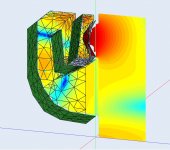
1) The shape seems to be defined with nodes rather than a mesh file. How are they importing these node points? The cabinet shape looks too complicated to just be working it out on a post-it note without CAD.
2) How does one know when to use an additional internal domain? Here we see multiple sections of the horn get their own internal domain, but I do not understand what necessitates the split at those specific sections. Why can't the horn be a single internal domain?
The example file 'Speaker Cabinet Bass-Horn Bogart' looks like a good learning candidate. However I have a couple of questions:
1) The shape seems to be defined with nodes rather than a mesh file. How are they importing these node points? The cabinet shape looks too complicated to just be working it out on a post-it note without CAD.
2) How does one know when to use an additional internal domain? Here we see multiple sections of the horn get their own internal domain, but I do not understand what necessitates the split at those specific sections. Why can't the horn be a single internal domain?
Attachments
Hi Tenson, sorry I can't be more helpful, would also like to know when to apply a subdomain.
I find it quite easy to enter objects as a mesh file using fusion360 to model. I use the unstitch command to break down solids into shells, export to .step and then use GMESH to generate version II mesh files (.msh). This is a lot easier than using manualy calculated nodes (how I did my first simulations).
I find it quite easy to enter objects as a mesh file using fusion360 to model. I use the unstitch command to break down solids into shells, export to .step and then use GMESH to generate version II mesh files (.msh). This is a lot easier than using manualy calculated nodes (how I did my first simulations).
I'd like to use AKABAK to investigate an unwanted resonance a transmission line speaker.
A linear acoustic BEM code isn't the right tool for this type of study. The effect of the damping material in the line will be missing. This will not only lead to an incorrect Q for the resonance but also an incorrect frequency because the damping material changes the effective speed of sound in the line. More seriously, if the resonance involves incompressible fluid motion (e.g. Helmholtz resonance) the relevant terms will not be present in the sourceless linear wave equation used in a linear acoustic BEM code. In addition, for long thin internal shapes the numerical error in the boundary integral evaluated by BEM code can become large and swamp the answer. This can be checked and possibly got around.
A reliable simulation would need to include both the physics of the damping material and possibly relevant incompressible motion. The 1D network models often used to simulate transmission lines usually include this physics but, obviously, don't include any 2D or 3D effects which may be relevant. To include everything you would need to use a low Mach number CFD code or an incompressible CFD code with an acoustic code that can use the CFD predictions to construct the relevant source terms. For example, look at what the various types of numerical methods are used for by KEF here.

Thanks Andy, I did read your comments earlier and hoped you might chime in.A linear acoustic BEM code isn't the right tool for this type of study. The effect of the damping material in the line will be missing. This will not only lead to an incorrect Q for the resonance but also an incorrect frequency because the damping material changes the effective speed of sound in the line. More seriously, if the resonance involves incompressible fluid motion (e.g. Helmholtz resonance) the relevant terms will not be present in the sourceless linear wave equation used in a linear acoustic BEM code. In addition, for long thin internal shapes the numerical error in the boundary integral evaluated by BEM code can become large and swamp the answer. This can be checked and possibly got around.
A reliable simulation would need to include both the physics of the damping material and possibly relevant incompressible motion. The 1D network models often used to simulate transmission lines usually include this physics but, obviously, don't include any 2D or 3D effects which may be relevant. To include everything you would need to use a low Mach number CFD code or an incompressible CFD code with an acoustic code that can use the CFD predictions to construct the relevant source terms. For example, look at what the various types of numerical methods are used for by KEF here.
I can't pretend I really understand the mathematical limits of BEM vs CFD. Any way you can try to explain in laymen's terms?
What you said makes me think maybe BEM is not very accurate where wave velocity approaches zero (and pressure is maximum), such as at the actual boundaries?
I have installed Salome, but am still getting my head around AKABAK.
My aim is locate the velocity mode of the ~1KHz resonance in the line so I can add a 'tap' there to kill it off. Perhaps the most practical way to do this is find a very small microphone module and run it down the line on a wire. The line cross-section is only 6mm x 100mm so I need something like a MEMS mic.
I'd still love to understand when and where multiple internal domains are required.
Perhaps the classical example of a Helmholtz resonance is steadily blowing over the top of a milk bottle. If you were to perform a BEM simulation of this case the predicted result would be silence because there is no varying motion to create sound on the boundary (the blowing being steady). The air motion that creates sound is occurring within the solution region not at the boundary and so you need to use a numerical method that grids the solution region and also includes the terms for the air motion that is not sound.
The full motion of air is given by the Navier-Stokes equations which are 5 equations expressing the conservation of mass, momentum and energy. This is extended and complicated a bit by the presence of both air and fibres in the regions of sound absorbing material but it still involves mass, momentum and energy of the two phases plus a bit of empiricism on how they interact. This is what you need but CFD codes that include the lot and handle sound accurately at low Mach numbers are rare.
Curiously one can express the Navier-Stokes equations as a single equation with the linear wave equation involving a single variable on one side of the equals sign and a whole bunch of complicated terms involving all 5 variables on the other side of the equals sign. This is the Lighthill equation. An acoustic BEM method approximates the full equations by setting all the complicated source terms to zero and retaining only the wave equation and a single acoustic variable. This is a huge approximation but useful when the only thing going on is sound which enters or leaves via the boundary and is not created or absorbed within.
CFD codes have difficulties including sound accurately at low Mach numbers which is the case for the air motion inside a TL speaker. The most common way round this is to assume the flow is incompressible which removes all sound waves. These are generally referred to as incompressible CFD codes. Curiously because sound waves are weak compared to other fluid motions (e.g. 100 dB sound involves pressure variation of the order of 1 Pascal whereas the background pressure is of the order 100000 Pascal) it turns out the 5 variables predicted by an incompressible CFD code can be used to accurately evaluate all the source terms in the Lighthill equation neglected in the linear wave equation.
This leads to the common approach of using a CFD code to study the air motion without sound (or sometimes inaccurate sound) and then solving a linear wave equation with source terms evaluated from the CFD predictions. This is usually an acoustic finite element/volume/difference code which grids the whole volume. This two step process means sound cannot influence the non-acoustic fluid motion which is usually a good assumption when the sound level is low enough to be essentially linear. However, there are cases where a low level linear sound repeatedly weakly nudges a non-acoustic motion in the same way until it grows over time into a significant motion (e.g. fat lady singing breaking a wine glass) so the assumption needs watching.
Before chasing down CFD codes and acoustic codes that include source terms. Is your 1 kHz resonance one of the higher order line modes? Is the frequency close to that for one of the dimensions like the width of the line?
Perhaps the classical example of a Helmholtz resonance is steadily blowing over the top of a milk bottle. If you were to perform a BEM simulation of this case the predicted result would be silence because there is no varying motion to create sound on the boundary (the blowing being steady). The air motion that creates sound is occurring within the solution region not at the boundary and so you need to use a numerical method that grids the solution region and also includes the terms for the air motion that is not sound.
The full motion of air is given by the Navier-Stokes equations which are 5 equations expressing the conservation of mass, momentum and energy. This is extended and complicated a bit by the presence of both air and fibres in the regions of sound absorbing material but it still involves mass, momentum and energy of the two phases plus a bit of empiricism on how they interact. This is what you need but CFD codes that include the lot and handle sound accurately at low Mach numbers are rare.
Curiously one can express the Navier-Stokes equations as a single equation with the linear wave equation involving a single variable on one side of the equals sign and a whole bunch of complicated terms involving all 5 variables on the other side of the equals sign. This is the Lighthill equation. An acoustic BEM method approximates the full equations by setting all the complicated source terms to zero and retaining only the wave equation and a single acoustic variable. This is a huge approximation but useful when the only thing going on is sound which enters or leaves via the boundary and is not created or absorbed within.
CFD codes have difficulties including sound accurately at low Mach numbers which is the case for the air motion inside a TL speaker. The most common way round this is to assume the flow is incompressible which removes all sound waves. These are generally referred to as incompressible CFD codes. Curiously because sound waves are weak compared to other fluid motions (e.g. 100 dB sound involves pressure variation of the order of 1 Pascal whereas the background pressure is of the order 100000 Pascal) it turns out the 5 variables predicted by an incompressible CFD code can be used to accurately evaluate all the source terms in the Lighthill equation neglected in the linear wave equation.
This leads to the common approach of using a CFD code to study the air motion without sound (or sometimes inaccurate sound) and then solving a linear wave equation with source terms evaluated from the CFD predictions. This is usually an acoustic finite element/volume/difference code which grids the whole volume. This two step process means sound cannot influence the non-acoustic fluid motion which is usually a good assumption when the sound level is low enough to be essentially linear. However, there are cases where a low level linear sound repeatedly weakly nudges a non-acoustic motion in the same way until it grows over time into a significant motion (e.g. fat lady singing breaking a wine glass) so the assumption needs watching.
Before chasing down CFD codes and acoustic codes that include source terms. Is your 1 kHz resonance one of the higher order line modes? Is the frequency close to that for one of the dimensions like the width of the line?
Thanks for your detailed reply Andy!
I'm sorry to say most of this still goes way over my head when you are talking about equations.
I have wondered and I don't know if my question is even 'right' but I'll ask anyway. What does BEM typically model as an 'input signal' from which it derives all the other factors such as frequency response, pressure, velocity? What I mean by this is does it solve for a step response that would represent a single forward motion of a diaphragm or is the input sinusoidal like an impulse? Does it solve for velocity and then derive pressure, or the other way?
FWIW you can set a wall impedance in AKABAK to represent some absorption.
If the pressure and particle velocity are known over all the boundaries of a region then the sound at any point within the region can be evaluated by essentially adding up all the contributions from all the boundaries. This is the second stage of a BEM method where the fields are evaluated.
In the first stage of a BEM method the user must specify over all the boundaries a pressure, a velocity or the ratio of pressure and velocity (impedance). The user can change what is specified on different parts of the boundary but the whole boundary must have one and only one quantity specified. This is the input along with the geometry, frequency and properties of the air. The BEM method then solves to determine the quantity that was not specified. (Strictly there is only one acoustic variable and it's gradient but it is clearer using pressure and particle velocity for illustration).
A typical acoustic BEM code like AKABAK (there are variations) assumes simple harmonic motion and determines the acoustic field for a single frequency. To obtain a Frequency Response Function requires repeating the calculation for different frequencies and possibly different conditions on the boundary depending on what is being modelled. There is no equivalent to modal analysis with acoustic BEM making it fairly computationally expensive in comparison with, say, obtaining the FRF for the cabinet to use to specify input velocities for the BEM simulation.
Okay that makes sense I think - like calculating each point on the surface as a sound source and how they interreact. Like beam forming.If the pressure and particle velocity are known over all the boundaries of a region then the sound at any point within the region can be evaluated by essentially adding up all the contributions from all the boundaries. This is the second stage of a BEM method where the fields are evaluated.
How does the user know what that quantity will be over each part of the boundary? Presumably this is complex when we have a radiating sound source and 3D geometry.In the first stage of a BEM method the user must specify over all the boundaries a pressure, a velocity or the ratio of pressure and velocity (impedance). The user can change what is specified on different parts of the boundary but the whole boundary must have one and only one quantity specified.
A typical acoustic BEM code like AKABAK (there are variations) assumes simple harmonic motion and determines the acoustic field for a single frequency. To obtain a Frequency Response Function requires repeating the calculation for different frequencies and possibly different conditions on the boundary depending on what is being modelled. There is no equivalent to modal analysis with acoustic BEM making it fairly computationally expensive in comparison with, say, obtaining the FRF for the cabinet to use to specify input velocities for the BEM simulation.
Thanks for taking the time to educate me and anyone reading this!
How does the user know what that quantity will be over each part of the boundary? Presumably this is complex when we have a radiating sound source and 3D geometry.
Velocity is the commonly chosen quantity with speakers since this is known by the user. On the surface of an inert cabinet it is zero. Over a rigid cone it is a constant value. For a bending cone or vibrating cabinet the velocity varies over the surface and is usually obtained from a FEM simulation of the cone or vibrating cabinet. A few codes can write out values over parts of the boundary in a format recognised by the BEM solver but usually the user needs to create a short script to transfer the required values for each frequency (the velocities generally being different at different frequencies). Normally such scripts will have been created in the past for earlier simulations and so one tends to modify an old script which is usually pretty quick. First time it will take a while though to work out how to do it and then write the script.
There are some rules of thumb mentioned in the AKABAK3 help file (moreso than ABEC3, with recent updates), the “SP38”, “Bogart45” and “ABEC21 Sealed” example models, plus a couple of papers by the developer Joerg Panzer:Hi Tenson, sorry I can't be more helpful, would also like to know when to apply a subdomain.
Panzer, Jörg W. 1997. “Simulation of Complex Loudspeaker Enclosures.” AES, February. http://www.randteam.de/_Docs/Pub/aes_Euphonia_e.pdf.
(This one is about classic AKABAK, but the diagram that displays when each lumped element is used in series or parallel gives a good indication of when you may want to apply a subdomain division.)
Panzer, Joerg “Boundary Element Method of of AKABAK.” Accessed June 4, 2021. http://www.randteam.de/_Docs/AKABAK/Studies/AKABAK-BEM.pdf.
Panzer, Joerg. 2012. “Coupled Lumped and Boundary Element Simulation for Electro-Acoustics.” In Proceedings of the Acoustics 2012 Nantes Conference. Hal-00811256. https://hal.archives-ouvertes.fr/file/index/docid/811256/filename/hal-00811256.pdf.
Panzer, Joerg. 2020. “Boundary Element Subdomain Modeling for Electroacoustic.” In Audio Engineering Society Convention 149. Audio Engineering Society. http://www.aes.org/e-lib/download.cfm?ID=20970.
A good way to think about it is that subdomains each represent a relatively stable acoustic field behaviour. If there’s a significant change in a section’s volume or direction, then that’s a good indication that breaking it down into subdomains is needed for improved accuracy. The simple 2D BEM example of a duct with bend here uses two subdomains, for example:
https://randteam.de/_Docs/AKABAK/Studies/AKABAK-BEM.pdf
This set of presentation slides also highlights the possible differences in resonance details mentioned by @andy19191 in BEM sims versus reality. Check the measurement comparisons:
Likewise, any section that is relatively narrow should have its own subdomain with correctly set meshing parameters to avoid overlapping of calculation point radius from the centre of each mesh element - see the latest version for a nice visual example in the help under Meshing, plus a relatively new pink highlight when the solver detects this error.
Anyone care to help out with "importing" my old .aks scripts into the new Akabak 3 ? The help file didn't go into enough detail (for me) to get it done.
Hello again, I'm back!
Is it possible to implement a FIR filter in AKABAK simulations?
I want to simulate 3 identical drivers where two of them reduce in level with a linear phase response to control directivity of the array. If I could import a filter impulse from RePhase that would be great.

Is it possible to implement a FIR filter in AKABAK simulations?
I want to simulate 3 identical drivers where two of them reduce in level with a linear phase response to control directivity of the array. If I could import a filter impulse from RePhase that would be great.
So I found it IS possible to do a linear phase filter at least in the new akabak by simply inserting the 'filter' block and there is a 'linear phase' option that can be enabled.

Last edited:
Does anyone know how to utilise biquad coefficients in the Filter block in AKABAK?
Coefficients generated elsewhere (e.g. from VituixCAD or https://www.earlevel.com/main/2021/09/02/biquad-calculator-v3/) don't seem to translate/work well when defined in the Formula area of the Filter block.
There is an example for Linkwitz-Riley in the software, but it's very basic, and the coefficients there don't translate to other software.
Feel like I'm missing something basic here.
I am not 100% sure as I had not tested it, but probably it is possible to get biquad coefficients to filter with Formula option, basically you need to write transfer function with biquad coefficients.
Other tested way is Data file option, you need to create with some other tool SLP and phase data containing file and import it to AKABAK and attache in Data file option to LEM filter.
Other tested way is Data file option, you need to create with some other tool SLP and phase data containing file and import it to AKABAK and attache in Data file option to LEM filter.
Anyone working with Akabak and dipol / ripol simulations? I've a basic question about internal and external in BEM. As I understand, for an open system like OB, dipol or ripol, anything is internal, except the room. Including all parts of the cabinet / baffle. Am I right or wrong?
Anyone working with Akabak and dipol / ripol simulations? I've a basic question about internal and external in BEM. As I understand, for an open system like OB, dipol or ripol, anything is internal, except the room. Including all parts of the cabinet / baffle. Am I right or wrong?
It depends on which domain/s you choose to simulate and how you choose to subdivide those domains if at all.
For example, an open baffle speaker in an anechoic space consists of two domains: the air is the external domain and the solid (baffle, drivers,...) is the internal domain. You would normally set akabak up to simulate the sound in the external air domain.
A ported speaker in an anechoic space also has two domains: an internal solid one and an external air one which includes the air inside the speaker via the port. However, BEM can have some numerical accuracy issues if this single external air domain is treated as a single domain and so it will usually be subdivide into 2 or 3 coupled external domains such as one for inside the speaker, one for inside the port and one for outside the speaker.
If you choose to simulate the sound of a speaker in a room then the air in the room is an internal domain with whatever is outside the room an external domain. This makes the solid of the speaker also part of the external domain. In this case you would set akabak up to simulate the air in the room as an internal domain.
Thank you for the fast answer. But I'm still struggling with the concept.
I've created one subdomain for the speaker and one for the environment (let's start with free air for simplification). I've connected both with and interface than contains 3 elements, representing the openings of the box. I've expected that baffles and elements, defined as reflective, are strict boundaries. Except the interfaces. But it looks like I'm totally wrong. 🤔
Do I have to build separate fron/rear subdomains?


But the mic curve goes into the expected directiom, including the resonance peak at 400Hz.

I've created one subdomain for the speaker and one for the environment (let's start with free air for simplification). I've connected both with and interface than contains 3 elements, representing the openings of the box. I've expected that baffles and elements, defined as reflective, are strict boundaries. Except the interfaces. But it looks like I'm totally wrong. 🤔
Do I have to build separate fron/rear subdomains?
But the mic curve goes into the expected directiom, including the resonance peak at 400Hz.
Attachments
- Home
- Design & Build
- Software Tools
- AKABAK 3