Good job! That's a good starting point. I didn't know about the Python scripting in FreeCAD - just anything should be possible with that. I will also give it a try, I only hope this will be the last time I have to learn some new CAD 😱
I was able to hack the code to make two separate wires by splitting the coordinate files and reading each in separately. This could be extended to all the files but is very ugly.
Using that code creates a polyline of straight segments between the points. That wire then needs to be turned into a BSpline, so the curves can be lofted properly. There is no scripting function for that so it would need to be done manually which is not hard but not elegant either 🙂
The BSpline can be created directly by specifying their vectors
Code:
import FreeCAD, Draft

p1 = FreeCAD.Vector(0, 0, 0)
p2 = FreeCAD.Vector(1000, 1000, 0)
p3 = FreeCAD.Vector(2000, 0, 0)

BSpline1 = Draft.makeBSpline([p1, p2, p3], closed=True)
I imagine for you it might be easier to modify Ath to have it spit out a macro with the vectors formatted directly to create the BSplines to save writing and reading them separately.
As I quickly ran out of talent on the coding front I was able to get Rhino to make a surface by importing the point cloud data and creating curves through the points of each slice before lofting them together. A bit of manual effort but no coding required.
Attachments
But it is possible, has to be. It's just that this transfer matrix is not known "modally" in the numerical case, but it is in the analytical case, i.e. OSWG. But one could make up this matrix numerically by calculating the far field for each possible mode shape at the throat. You know the zeroth order one already, but you don't know the higher order ones.
If you expand the throat as a series of functions, all known in this case (Bessel functions), and then calculate the far fields numerically for each mode shape > 0, doing this for say the first four or five modes, then you would have the matrix that you need to back calculate the throat wavefront shape from the far field data. If that's what you want to do.
Thanks, yes, I guess - I still have only a hazy idea of the actual mathematical proceeding that would need to follow, however.
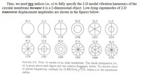
When you say "first four or five modes", what modes do you actually mean? I still don't understand this ordering of (m,n) 😱
I'm trying to get into this but it's difficult. I'll probably leave it at manufacturing the PWT (still waiting - there's so much other work during the summer).
https://courses.physics.illinois.ed...P406POM_Lecture_Notes/P406POM_Lect4_Part2.pdf
Attachments
Yeah, I already looked at the FreeCAD scripting and it seems very nicely done. It should be easy to integrate Ath output into FreeCAD, at least if all the commands work as expected - I did no practical testing yet....I imagine for you it might be easier to modify Ath to have it spit out a macro with the vectors formatted directly to create the BSplines to save writing and reading them separately.
Thanks, yes, I guess - I still have only a hazy idea of the actual mathematical proceeding that would need to follow, however.
When you say "first four or five modes", what modes do you actually mean? I still don't understand this ordering of (m,n) 😱
I'm trying to get into this but it's difficult. I'll probably leave it at manufacturing the PWT (still waiting - there's so much other work during the summer).
Those modes are similar, but different because the boundary conditions are different. The membrane has clamped (v=0) conditions at a, while the throat aperture would b zero slope (dv/dr = 0). The m and n refer to the axisymmetric modes m and the non-axi mode n. In our problem the greatest variation will only be radial, so we would need only the first four or five m modes. (The extension to non-axi is easy once you understand the axisymmetric. So the functions will be J0(km * a) where km is determined such that J0(km * a) has a zero slope at a.
Thus you can see that what you have now are the J0(km * a) where in this case the km is zero - hence the aperture wavefront is assumed to be flat.
If one expands the throat aperture in a set of orthogonal functions (as described) then the far field response will also have a set of orthogonal functions (but in the numerical case we don't know those.) This means that there is a one-to-one relationship between the modes in the aperture and those in the far field. Expand the far field into the as yet unknown functions and we then know the modes in the aperture.
Take for example an OSWG. The mouth flare is a problem, but if we made a very long OSWG then we could measure inside of the device well away from the mouth and thus find the aperture curvature because we know the modes inside of the device. But the far-field is contaminated by the mouth flare.
It's not really a practical solution and probably not nearly as effective as a PWT, but it is doable. The PWT works because we also know the internal modes for that situation.
My bad, I didn't fully noticed that the picture was for a clamped membrane. Whether you meant only the axisymmetric modes was what I wanted to really ask. Thanks.
OK, I will try to finish the PWT - almost done in fact. I'm really curious what can be done about that.
I have it designed so that the driver can be mounted in several rotated positions easily (in steps of 30 or 45 deg), just in case it's needed.
OK, I will try to finish the PWT - almost done in fact. I'm really curious what can be done about that.
I have it designed so that the driver can be mounted in several rotated positions easily (in steps of 30 or 45 deg), just in case it's needed.
Last edited:
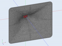
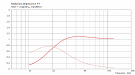
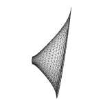
Back to the Ath 4.6 for a while, this is a simple example how different profiles can be blended together.
These are the profiles (red=horizontal; blue=vertical):
This is the definition file with both profiles blended:
These are the profiles (red=horizontal; blue=vertical):
This is the definition file with both profiles blended:
Code:
[FONT="Courier New"]Geometry.Definition = 1
Throat.Profile = 1
Throat.Diameter = 25.4 		; [mm]

[b]; Fixed parameters[/b]
Throat.Angle = 7 			; [deg]
Length = 94				; [mm]
Term.q = 0.996

[b]; Horizontal profile[/b]
;Coverage.Angle = 45
;Term.s = 0.7
;Term.n = 4.0

[b]; Vertical profile[/b]
;Coverage.Angle = 18
;Term.s = 1.08
;Term.n = 2.55

[b]; Blended profile[/b]
Coverage.Angle = 45 - 27*sin(p)^2
Term.s = 0.7 + 0.38*sin(p)^2
Term.n = 4.0 - 1.45*sin(p)^2

Morph.TargetShape = 1
Morph.FixedPart = 0.0
Morph.Rate = 3
Morph.CornerRadius = 18 ; [mm]
[/FONT]
Attachments

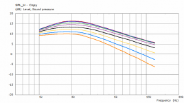
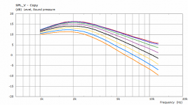
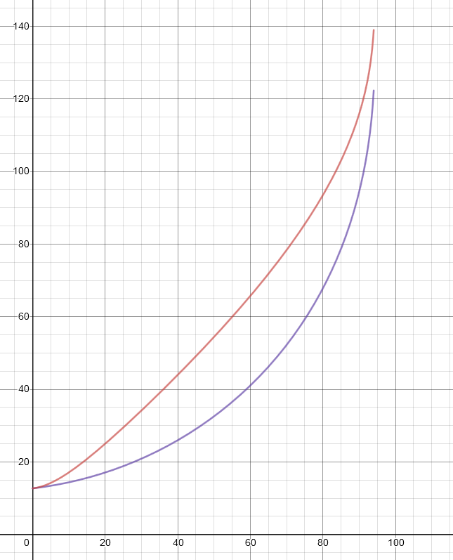
BTW, I haven't seen any occasional spikes in the simulated curves for quite a long time, maybe since 4.6. I believe this is because I fixed some inconsistencies in the mesh structure - there used to be the same points defined twice in some cases. This is no longer the case. The above results were obtained for mesh resolution of 4 and 8 mm (i.e. throat and mouth resolution respectively).
- The above waveguide is only 278 x 246 x 94 mm big.
- The above waveguide is only 278 x 246 x 94 mm big.
Last edited:
hey Mbat, is it possible to use the direct formula (with the p angle term) to make a profile with different angles in the same plane? (kind of like some pa horns use for amplitude shading) gave it ago, but hadn't found a smooth curve which gives a shape like that yet
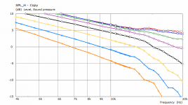
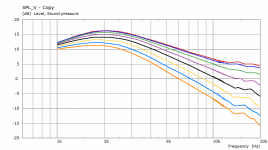
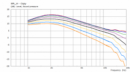
From time to time I also run the simulation for 10k - 20k with an increased resolution (4 mm for the whole mesh in this case). The two sets of curves overlap between 10 and 12 kHz here:

Here you can see the approximate error you can expect...
Here you can see the approximate error you can expect...
Attachments
Sorry, I don't get what you mean by that.hey Mbat, is it possible to use the direct formula (with the p angle term) to make a profile with different angles in the same plane? (kind of like some pa horns use for amplitude shading) gave it ago, but hadn't found a smooth curve which gives a shape like that yet
Ah, this doesn't make a flat mouth. So I guess the proper solution would be skewing a guiding curve set as the mouth outline. I can think about implementing this.
Last edited:
Ah, this doesn't make a flat mouth. So I guess the proper solution would be skewing a guiding curve set as the mouth outline. I can think about implementing this.
Thanks for the ideas! yeah the example posted was similar to what I was thinking.
i'm not really sure its a feature worth having. To be honest i was more curious if the approach is even worth it, or if it has a bunch of downsides apart from worse pattern flip.
From time to time I also run the simulation for 10k - 20k with an increased resolution (4 mm for the whole mesh in this case)....
Here you can see the approximate error you can expect...
Not something to worry about, I guess?
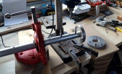
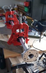
Impressive work on the tube btw.
It's steel?
Last edited:
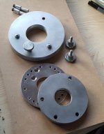
Would probably be quite difficult to make those holes in steel with what appears to be a brad point bit.Not something to worry about, I guess?
Impressive work on the tube btw.
It's steel?
It is. The only hole that goes through the tube is ⌀2 mm (i.e. the same diameter as the hole on the WM61 capsule) about 1.5 mm deep, the rest is blind. I thought that the more intact the inner wall remains the better. Otherwise there would be ⌀8 mm holes for six mics. We'll see how that goes....what appears to be a brad point bit.
- Home
- Loudspeakers
- Multi-Way
- Acoustic Horn Design – The Easy Way (Ath4)