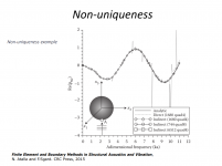
Regarding non-uniqueness mitigation methods, this is what ABEC's documentation says:
"In ABEC experiments were done implementing the CHIEF [25], Burton and Miller [26] and the Dual Surface Method [27]. A good compromise of calculation speed, stability and accuracy in the given context provides the Dual Surface Method. The other method may follow for final implementation at a later stage."
25. Schenk, H: Improved integral formulation for acoustic radiation problems, JASA 44, Dec 1967
26. Burton, A; Miller, G: The application of integral methods to the numerical solution of some exterior boundary-value problems, Proc Roy Soc London A 323, 1971
27. Mohson, A; Piscoya, R; Ochmann, M: The application of the dual surface method to treat the nonuniqueness in solving acoustic exterior problems, Acta Acoustica, Vol 97, 2011
So, obviously, it was addressed. I don't remember if I ever used this feature (NUC=true in Control_Solver).
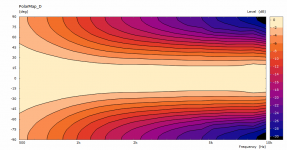
So what is your take on that?... Now the weirdness shows up vertically when it was horizontal before
That it is not real or that it is an exaggeration of a minor issueSo what is your take on that?
I will give it try with the NUC=true in the Control Solver as it was not included in these sims.
That seems a likely explanation, Dimitrij.
NUC is mentioned in a lot of horn-related research literature, including the thesis of M. Makarski.
Yes, it is common problem in BEM. I also faced NUCs by modeling horns in Axidriver, where narrow sharp peaks also appeared.
Btw bear in mind, that if you set NUC=true in Abec3 to overcome the NUC problem the calculations last considerably longer (by a factor of 2, if I am correct).
For those interested in the paper by Mohson, A; Piscoya, R; Ochmann, M: The application of the dual surface method to treat the nonuniqueness in solving acoustic exterior problems, Acta Acoustica, Vol 97, 2011.
Attachments
Why exactly 198 mm? 🙂... How about the same mouth (484 x 418) x 198 mm + 1.4" ?
I can try it later. I actually came to like somewhat lower DI (i.e. shallower) designs as they naturally allow for a smaller woofer, like 12".
Last edited:
"In Section 3.4.2 the effects of the non-uniqueness of the solution of the interior Laplace problem with a Neumann boundary condition were discussed. The boundary integral Equations have a similar property at the characteristic wavenumbers, and this is also often termed the non-uniqueness problem.
Although it is ‘unlikely’ in practice that the value of wavenumber k is equal to a characteristic wavenumber k*, it is shown in Amini and Kirkup that the numerical error as a consequence of being ‘close’ to a characteristic wavenumber is O(1/|k-k*|). Hence, one technique of resolving the problem is to use finer meshes in the neighbourhood of the characteristic wavenumber in order to offset this error. However, this strategy is likely to be prohibitive, requiring the overhead of creating a range of meshes and increased computational cost. The values of the characteristic wavenumbers are also generally unknown, although they can be found (as discussed in Section 4.2), but at a substantial computational cost. It is also found that the characteristic wavenumbers cluster more and more as the frequency
increases. In conclusion, therefore, the boundary integral equations are—in practice—only useful for frequencies reasonably below a conservatively estimated first characteristic wavenumber, severely restricting the methods to the low frequency range in practice."
From:
Attachments
Last edited:
That's also easily possible - to generate a second, much finer mesh and run the calculation just for the problematic narrow range(s) of frequencies... (if that actually helps). I'm only not sure how easy would it be to stitch the data together in VACS.
Last edited:
Why exactly 198 mm? 🙂
I can try it later. I actually came to like somewhat lower DI (i.e. shallower) designs as they naturally allow for a smaller woofer, like 12".
Because I prefer to keep the 8 and thought 200mm would be a nice depth (limit)

Last edited:
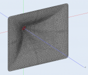
Has anyone tried to divide the interior into several sub-domains (more than one)? I guess it could reduce the computation time, especially for larger horns.

Attachments
Last edited:
Were both sims executed with the option NUC=true?
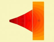
It's likely the leftover artefacts disappear with an even denser mesh.
Apart from that, it looks promising.
It's likely the leftover artefacts disappear with an even denser mesh.
Apart from that, it looks promising.
Last edited:
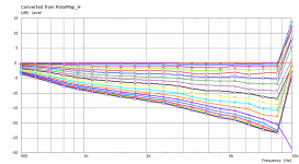
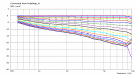
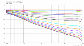
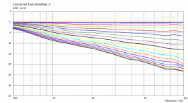
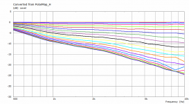
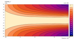
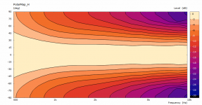
The previous polars were derived from the far-field polar maps ("Graph - Convert curves <-> contour" feature in VACS).It's likely the leftover artefacts disappear with an even denser mesh.
This is a comparison between polars at 2.5 m for the coarse and the finer mesh. This is also the reason I try to keep the mesh density at minimum - typically it makes a little difference for the most part.
Attachments
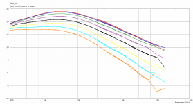
Differences are very small indeed, though the finer mesh pushes the ripples higher up, it seems.
That's how it works. If you wanted to calculate up to 20 kHz you would need a much finer mesh but it would be a total waste of time and power to solve it for lower frequencies. Maybe I should really try to create at least two meshes at different densities, divide the frequency range of interest and compose that results.
Last edited:
OK, now it's a bit better. No more questions 🙂


Attachments
- Home
- Loudspeakers
- Multi-Way
- Acoustic Horn Design – The Easy Way (Ath4)