Hello EucyHi Christian... I'd be interested in seeing your exciter model if you're agreeable
Eucy
The model schematic and parameters for DAEX25FHE, DAEX25VT, XT25, XT32 are now in the document Github exciter_characteristics.pdf
@Veleric : Thank you Eric for the measurements.
Extract :

Thanks Christian/Eric - I note some reasonable differences in measured vs published rms values for the Xcite 24-4 and 32-4 units...
Eucy -
Eucy -
The values from the measurements and from the specification are comparable only if they refer to the same model. The model being like the way to extract several information from the impedance curve. So in this paper only the value from the first page are comparable directly referring to the Thiele and Small (T/S) parameters (or model) which suppose a constant Rms value over the frequency range.I note some reasonable differences in measured vs published rms values for the Xcite 24-4 and 32-4 units...
The model in last page (the one I posted just before) suppose a frequency dependent Rms
From this table it comes as resonance frequency for XT25 326Hz (for 306Hz in the spec), for XT32 310Hz (for 312Hz in the spec) so using those frequencies for Rms calculation in last page , it comes for XT25 0.175 vs 0.09 in the spec and 0.14 in T/S model and for XT32 0.31 vs 0.2 in the spec and 0,2 in T/S model.
Knowing since those measurements that the damping is probably the parameter with the most important error margin, I would say it is not that bad.
With your comment, I see the lines "Rms VC / magnet" and "Mms VC / magnet" of the first table are not consistent. They are now more clearly split (I uploaded a new version of the file)
The main comment I would do is about XT25 which is much stiffer at 0.12mm/N the the Dayton models FHE, VT at 0,4mm/N. I don't know the consequence. The XT32 is comparable (from those parameters) to the DAEX30HSFE.
Christian
Christian,The main comment I would do is about XT25 which is much stiffer at 0.12mm/N the the Dayton models FHE, VT at 0,4mm/N. I don't know the consequence. The XT32 is comparable (from those parameters) to the DAEX30HSFE.
Looks like they slipped a few digits in the Dayton specs for Cms, unless they are a lot stiffer than we think. Presumably they mean m/N instead of mm/N. Or am I missing something? Your numbers make more sense to me!
Eric
Hello Eric,Looks like they slipped a few digits in the Dayton specs for Cms, unless they are a lot stiffer than we think. Presumably they mean m/N instead of mm/N. Or am I missing something? Your numbers make more sense to me!
Yes it is a mistake in the datasheet. We can confirm ss the fs is visible on the impedance curve, the mms makes sense in gram range so if you compute the cms it comes below 1mm/N. fs = 1/2/pi/sqrt(mms*cms)
@EarthTonesElectronics
Dave,
In PETTaLS, have you implemented a frequency dependent Q? If yes, is it possible to know which law? Thank you
Christian
Dave,
In PETTaLS, have you implemented a frequency dependent Q? If yes, is it possible to know which law? Thank you
Christian
Agh - You guys are sucking me in to all this stuff - 🤓 - I've been hunting around all the complexities we haven't yet covered - one of them being frequency dependent stiffening of panel material and the effect on output - here's a taster for EPS to chew on - the zero line is the expected static FEA (or other) result - so below about 500Hz, static is pessimistic, and above it we can expect losses due to freq dependent stiffening. What a rabbit hole
Eucy
Eucy
Attachments
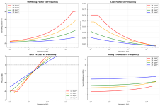
Hello Eucy,I've been hunting around all the complexities we haven't yet covered - one of them being frequency dependent stiffening of panel material and the effect on output - here's a taster for EPS to chew on - the zero line is the expected static FEA (or other) result - so below about 500Hz, static is pessimistic, and above it we can expect losses due to freq dependent stiffening.
From my side, I started from a list of common observations or questions I was able to list from our discussions : is the coincidence frequency a reality for a DIYer? which cause and countermeasure for the HF peak? which cause and countermeasure for the midrange peak from the rear side? why a simply hanging panel can be appreciated compare to other suspensions? what can be the benefit of added masses (edge, balance)? what are the suitable panel ratio and exciter location?... Far to be easy. The process is slow but some answers are here.
To come to your point, it is a piece of puzzle that doesn't fit in this set of questions. Or possibly I am not able to see how it fits.
Did you start from some observations or knowledge from an other domain for that?
Could you explain the plots and how they are related to each other?
The Young modulus is for sure a parameter but I think it the first time I see it frequency dependent. What is the source of this plot?
I can understand the loss factor even if damping is not implemented like that in my script. Its decrease with frequency makes also probably sense with my last observations about Depron (XPS). It is the reason of my question of the Q model to Dave.
The stiffening factor and the FR loss are new for me and I can't connect them at the moment to observations.
Christian
Hi Christian
I guess you may think this is a bit bleeding edge given the more obvious questions/problems we have to solve- but to me it is another peg in a hole relating to numerical analysis of the panels. So to explain the graphs a bit more - the whole revolves around the visco-elastic properties of EPS and XPS foam (and to a (significantly) lesser extent, but still applicable) timber - eg plywood. These materials display frequency dependent characteristics vis-à-vis stiffnesses, damping etc. (refs below). It looks like the fr loss/freq plot has been chopped a bit but the dotted zero line can be taken as the results of analysis using static properties. The material lines are corrections to be applied to these results based on freq dependent behaviour - ie correct low freq FR results upwards and high freq results downwards. Because these are material properties, the effects can't be applied by superposition but rather involve loopback processing - Can be done in FDM but more applicable to FEA.
Ref ( among others) :
https://www.researchgate.net/profil...anical-properties-of-expanded-polystyrene.pdf
https://www.researchgate.net/profil...t-strain-rates-and-different-temperatures.pdf
Zhou, J., & Lakes, R. S. (2004). Viscoelastic behaviour of closed-cell polymeric foams. Cellular Polymers, 23(3), 157–174.
https://link.springer.com/content/pdf/10.1007/s40891-021-00321-7.pdf
Hope this helps (a bit), and PS - your exciter model was very comprehensive - thanks
Cheers
Eucy
Thank you for the links Eucy. Frequency dependent material parameters is a key point for the simulation and the damping model is on the top of everythingHope this helps (a bit),
I'm glad to hear it. For the use I have of it in the FDM script it seems OK; pragmatic enough to get the parameters from a simple set of impedance measurements... and few lines of Python (or any language having a curve fitting function in its library)!and PS - your exciter model was very comprehensive - thanks
And I think the freq effects on our favourite plywood are significant enough to warrant investigation as well.
Eucy
Eucy
Not yet. We're working on it. It doesn't seem, at the moment, to be connected directly to a voice coil breakup mode, but I can't say for sure yet. There are quite a few voice coil breakup modes that we're measuring, and none of them seem to affect the output in this frequency range and to the same degree. The electromechanical model is not too complicated and seems to work well, but I don't actually know how to translate it into anything physical right now. This'll be something that I publish in a paper (eventually), so I don't want to speculate too much right now while it's still a bit of a mystery. It is definitely linked to the voice coil ring shape, and how the added circular stiffness affects the boundary conditions at the exciter-plate interface. This idea has been suggested to me several times in the peer review process, and I haven't ever taken a deep dive into it before.Excellent Dave.
Have you identified the component of this coupling resonance? Something linked to the voice coil structure?
I haven't - but you're touching on a good point: what's the right model for frequency-dependent Q factors? I would suggest that the correct interpretation is a mode-dependent Q adjustment factor, based on what percentage of the nodes or antinodes in the mode shape are touching the clamped or simply supported edges, which is obviously closely related to a frequency-dependent Q. This is something that I'll have to do more research on in order to find some general rules of thumb.@EarthTonesElectronics
Dave,
In PETTaLS, have you implemented a frequency dependent Q? If yes, is it possible to know which law? Thank you
Christian
Sorry about the delayed replies - this is a busy time for me!
Thank you for your answers Dave.I haven't - but you're touching on a good point: what's the right model for frequency-dependent Q factors? I would suggest that the correct interpretation is a mode-dependent Q adjustment factor, based on what percentage of the nodes or antinodes in the mode shape are touching the clamped or simply supported edges, which is obviously closely related to a frequency-dependent Q. This is something that I'll have to do more research on in order to find some general rules of thumb.
Sorry about the delayed replies - this is a busy time for me!
The Q factor and more generally the damping model is really a key point. When I started 2 years ago with FDM, and up to recently, I thought the difficulty was on the solver... but now the FMD solver is implemented and seeing your modal implementation, the damping is on the top of the difficulty list.
I just wrote a small script that tries to extract the Q factor from the mechanical admittance derived from an impedance measurement. Below is a plot for the plain polystyrene CCCC panel I shared some posts ago. The script is based on curve fitting. If you are interested, I can share the python code.
I implemented in it with a Q law able to increase the Q factor with a power of the frequency... on the few tests I have for now, it returned a constant Q value.
For the plain polystyrene it is Q = 33 in the plot below.
Question : in PETTaLLs, we see the Q factor seems to be chosen below what the impedance curve suggests. It is confirmed by my curve fitting script. Could you explain the reasons that lead you to adopt the PETTaLLS Q values?
Your model of damping by a constant modal Q factor is very smart; simple (at least in the idea) and efficient; and maybe unique among the publications dealing with plate vibrations. In parallel to a modal decomposition, the FDM script has the possibility of a direct frequency analysis which for now doesn't give good results because of the damping model. None of the classical damping models I tried are satisfactory and I haven't found papers making a link between a Q modal factor and a frequency model. By a frequency model I mean a model implemented in frequency approach of the main plate equation (the one with the 4th degree derivative). I am surprised that none of the models generally proposed in papers about plate vibrations don't fit to our experiments.
Question: do you know papers about plate damping that could help in a damping model suitable for our purpose?
Christian
Christian... I'm interested in which models you've tried and why you consider them to be no good...And in your curve fit code, the FDM script has the possibility of a direct frequency analysis which for now doesn't give good results because of the damping model. None of the classical damping models I tried are satisfactory and I haven't found papers making a link between a Q modal factor and a frequency model. By a frequency model I mean a model implemented in frequency approach of the main plate equation (the one with the 4th degree derivative). I am surprised that none of the models generally proposed in papers about plate vibrations don't fit to our
Cheers
Eucy
Eucy,Christian... I'm interested in which models you've tried and why you consider them to be no good...And in your curve fit code
My answer will be in 2 times. You will find below the information about the curve fit. I will provide you information about the damping models tested in a second time as it requests I explain a minimum to be more easily understandable.
So about the curve fit, of course it is provided as it is.
My scripts are not nice applications but more automated calculations so you have to put your hand in the Python code to run it.
Nothing special in it. All the power of this code comes from a curve fit function provided in the standard Python library Scipy. The detailed mechanism that optimize the parameter is in the library. The script provides the data and the model.
Attached you will find the draft of a paper I wrote to explain how to get the data and the model from the impedance curve and why. The explanation of how the exciter Rms is subtracted is not yet in it.
You will find also a zip file with 2 python files. One python file is the script, the second is a module called by the script that contains the exciter parameters (see the posts about exciter modelling).
I think there is no major difficulty to have it running on an other PC. Only of course Python and the needed libraries and some adaptation of the file path to the REW file according to your folder structure and OS (Linux for me).
It takes a few time to get the result of the curve fitting depending of the PC performance. There is nothing to show what happens during this period. Just be patient... I use a CPU load widget to get an idea of what happens.
Christian
Attachments
@Eucyblues99
Eucy,
I just used the script on an other material (PMMA with a file from Eric).
I detected a typo in one parameter on the DAEX25VT.
I modified the script. It has now the following parameters :

QPANEL_ONLY : set to True will remove the exciter Rms from the calculation giving the Q of the panel. False the Q will be global. (NEW)
FLOW : set a lower limit to search of peaks and to the curve fitting (NEW)
FHIGH : set an upper frequency. Already in the previous script but not as an easy to read parameter
HEIGHT : specify the minimum height of a peak. Already in the previous script but not as an easy to read parameter
PROMINENCE : set the minimum difference between 2 peaks. Already in the previous script but not as an easy to read parameter
QCONST : set to true to estimate a constant quality factor as expected by PETTaLS, False, Q will follow Q = Q0(1+ (f/f0)^k0)/2 which my current trial of a frequency dependent Q. NEW
2 remarks
If you want I run the script for you on some materials, send me your REW impedance files. It will go in the direction of a material library.
Christian
Eucy,
I just used the script on an other material (PMMA with a file from Eric).
I detected a typo in one parameter on the DAEX25VT.
I modified the script. It has now the following parameters :
QPANEL_ONLY : set to True will remove the exciter Rms from the calculation giving the Q of the panel. False the Q will be global. (NEW)
FLOW : set a lower limit to search of peaks and to the curve fitting (NEW)
FHIGH : set an upper frequency. Already in the previous script but not as an easy to read parameter
HEIGHT : specify the minimum height of a peak. Already in the previous script but not as an easy to read parameter
PROMINENCE : set the minimum difference between 2 peaks. Already in the previous script but not as an easy to read parameter
QCONST : set to true to estimate a constant quality factor as expected by PETTaLS, False, Q will follow Q = Q0(1+ (f/f0)^k0)/2 which my current trial of a frequency dependent Q. NEW
2 remarks
- You have to close the first graph (REW impedance and electrical elements of the model) then the second (admittance, peaks and limits) to reach the line where is the curve fitting. The result graph should appear.
- I have introduced a facto 1/2 in the frequency dependent Q
If you want I run the script for you on some materials, send me your REW impedance files. It will go in the direction of a material library.
Christian
Attachments
Eucy,Christian... I'm interested in which models you've tried and why you consider them to be no good..
Preparing an answer about damping leads me to see that I haven't explored all the values of the classical parameters... according to the papers I read, those parameters were expected positive while I just saw negative values make the job, at least part of the job.
All of that to say I have to investigate more. I don't forget your question.
Christian
Here are 2 new test cases of simulation (PETTaLS @EarthTonesElectronics , and my FDM python script)
Those test cases started from the idea to go further in the Q identification from the impedance measurements.
Eric made the measurements (tap test, REW) and the material parameters evaluation. Thank's a lot Eric!
In fact what started as a Q evaluation turned in a full tool chain evaluation.
The steps were as follow :
The very positive point is it was not necessary to tweak the parameters to get good results. They show also the possibilities to get the material parameters.
The simulations gave a good alignment in frequency. More difficult in impedance values.
The SPL outputs have also quite good similarities with the measurements.
The SPL curves are manually adjust in level to be superimposed. The check of the absolute level was out of scope.
The 2 test cases are summarized in the 2 attached pdf.
Below are the main outputs (impedance and SPL). Left are the plots with EPS, acrylic is on the right.
From the SPL, the low frequency SPL from the open back simulation in FDM is over-estimated. PETTaLs shows unexpected peaks (139 and 159Hz).
From the EPS impedance plot with PETTaLS, the lowest frequency peaks are not aligned with the measurement. The velocity maps at those frequency show some asymmetry (see pdf).
There shifts in the impedance plots because of the DC resistance which was not compensate.
Dave, if you want the files of this test, let us know.
Christian


Those test cases started from the idea to go further in the Q identification from the impedance measurements.
Eric made the measurements (tap test, REW) and the material parameters evaluation. Thank's a lot Eric!
In fact what started as a Q evaluation turned in a full tool chain evaluation.
The steps were as follow :
- tap tests with REW (panel alone)
- impedance and FR at 1m (panel with a DAEX25VT)
- estimation of the material parameters (Young modulus, Poisson's ratio) from the tap tests with FEA simulation
- quality factor extraction from the impedance measurement (see post before)
- for the FDM script, the impedance and FR from REW were exported in txt format to be used as references
- simulation
The very positive point is it was not necessary to tweak the parameters to get good results. They show also the possibilities to get the material parameters.
The simulations gave a good alignment in frequency. More difficult in impedance values.
The SPL outputs have also quite good similarities with the measurements.
The SPL curves are manually adjust in level to be superimposed. The check of the absolute level was out of scope.
The 2 test cases are summarized in the 2 attached pdf.
Below are the main outputs (impedance and SPL). Left are the plots with EPS, acrylic is on the right.
From the SPL, the low frequency SPL from the open back simulation in FDM is over-estimated. PETTaLs shows unexpected peaks (139 and 159Hz).
From the EPS impedance plot with PETTaLS, the lowest frequency peaks are not aligned with the measurement. The velocity maps at those frequency show some asymmetry (see pdf).
There shifts in the impedance plots because of the DC resistance which was not compensate.
Dave, if you want the files of this test, let us know.
Christian
Attachments
- Home
- Loudspeakers
- Full Range
- PETTaLS Flat Panel Speaker Simulation Software