Let me be clear. You want the impulse responses at the 14 angles that I use. Then you will put those into a polarmap? Using what software? If you mean you will import these into ARTA then yes that would be a good test.
I can plot at a fixed bandwidth smoothing, but I do not think that is the right way to do things in the long run, but for the purposes of this test it is fine.
I can't upload the Holm data because it is too large. What about E-mail?
I have really good data sets, which I believe that both pieces of software will work well, and I have some not so good data sets, which is where I see the largest deviations being likely. Which should we do?
Yes. I will read in the HOLM data for your chosen 14 angles(like I did for the Hansen data), select window to remove reflections, and then pad for 2048 point impulse files that get output in ARTA ready *.pir binary format. Takes just a few minutes, most of which is taken up selecting the window edges.Let me be clear. You want the impulse responses at the 14 angles that I use. Then you will put those into a polarmap? Using what software? If you mean you will import these into ARTA then yes that would be a good test.
For this comparison, I think sticking with 1/12 oct fixed bandwidth smoothing is best...would remove one potential source of differences.I can plot at a fixed bandwidth smoothing, but I do not think that is the right way to do things in the long run, but for the purposes of this test it is fine. I can't upload the Holm data because it is too large. What about E-mail?
Yes, sending HOLM files to my email would be just fine.
My preference would be one of each.I have really good data sets, which I believe that both pieces of software will work well, and I have some not so good data sets, which is where I see the largest deviations being likely. Which should we do?
One you expect to match well, and one you don't.
Just noticed your post#162 plot...Yes, that looks like it would be a good candidate.
What scale range should be used?
I had been using 30dB because I thought I remembered you mentioning that was your preference.
But looking at that last plot, is 35dB or 40dB more appropriate?
Whatever it is, we should use as close to the same range as possible.
ARTA provides range options in 5dB increments.
Last edited:
Thanks Earl and bolserst. I have the data in ARTA myself, but I figured I'd wait until Earl posted his Polar Map data to compare.
That 40° impulse is goofy, I'm not sure how I missed that. I had to manually click "Auto Detect" for the largest peak for the last 5 or 6 measurements because they were off by about 20ms. I hope to have a new speaker based on this design but with a cardioid midwoofer and an improved waveguide done before it gets too cold out. If I do I'll get my time lock issues in Holm sorted........I hope that's what's causing the gross difference in your result vs. ARTA!
That 40° impulse is goofy, I'm not sure how I missed that. I had to manually click "Auto Detect" for the largest peak for the last 5 or 6 measurements because they were off by about 20ms. I hope to have a new speaker based on this design but with a cardioid midwoofer and an improved waveguide done before it gets too cold out. If I do I'll get my time lock issues in Holm sorted........I hope that's what's causing the gross difference in your result vs. ARTA!
Nate
I can only figure that the time synch is the issue. I don't believe the results that I got either as I have never seen anything like that before. But then I always lock the synch so I am not likely to see what happens if you don't.
But I still don't follow why time synch does not work for you. I don't see how an external A/D convertor would make any difference, The sound cards all have A/D.
But I still don't follow why time synch does not work for you. I don't see how an external A/D convertor would make any difference, The sound cards all have A/D.
Yeah, but my D/A and A/D mic pre are totally separate devices, and I'm doing a good bit of processing on the PC (active xo). Holm sends the signal to the default Windows audio device, then my audio software "grabs" the stream for processing. Maybe that's not an issue. I've gotten it to work before though but it's been some time. Probably something fundamental I'm missing....I'll look into it.
I'll ask that you not post the result to your app since it's faulty. Thanks for your time Earl.
When you introduce DSP, like the crossover stuff above you will get additional delay through the electronics. On optimized DSP's I usually see at least 5-10 mS and in some cases over 50 mS. This can really fool some measurement software if its not expected.
In wireless system the extra time can be quite long (200-500 mS). Its good to look at the time between the electrical impulse and the acoustic impulse for both delay and stability of the delay.
In wireless system the extra time can be quite long (200-500 mS). Its good to look at the time between the electrical impulse and the acoustic impulse for both delay and stability of the delay.
I have regularly tested speakers through DSP units as active crossovers with no problem at all. But these have all been external to the PC. The PC grabbing the signal and processing it may be an issue.
Ok, so here is my speaker again:
- time locked after measuring zero degrees
- rotation around center of speaker
- measurement distance exactly 1.5m
- gate still only just above 4 ms (didn't raise my ceiling in the last couple of days)
- box volume: 100 l
- speaker f0: 50 hz
- speaker Qtc: 0.41
Raw holm data can be downloaded here:
One.com File Manager
Attachments
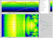
Here is a speaker that I just took data for last month. It has lots of serious problems that are all confirmed from the direct FFT data. How about we do this one?
Attachment #1: Comparison of problem speaker.
Attachment #2: Comparison of good speaker.
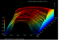
Attachment #3: Alternate visualization of good speaker.
Notes:
1) Data smoothing was 1/12 oct for both methods.
2) Scale range was 42dB for Gedlee polar map, and 40dB for ARTA sonogram.
Attachments
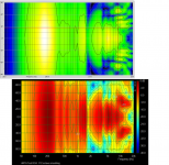

Bolserst Thanks for those plots. Not as different as I expected. Perhaps the ARTA stuff that I had seen in the past was heavily smoothed by the user rather by default in the software. I would have had no way of knowing which. But I have almost never seen an ARTA map as detailed as what is shown in your left hand plot. All of the real warts are there even if they aren't exactly the same. I think my technique works a little better near the 10 kHz point, but that is to be expected. But they are not so different that it would worry me.
For those who may not understand the above is how I and ARTA plot the exact same data sets. The data is identical in both examples between the two plots.
Do people prefer the RTA coloring or mine? I redid my color scheme after I read an article on using color in engineering plots. It was emphasized that it was important that the color scheme match what is being expressed and not just done willy-nilly or "colorful". So I ordered my color from bright to dull as intensity from high to low. ARTA is clearly not done this way as the highest levels are in a dark color with bright rings at an average level.
Ok, so here is my speaker again:
- time locked after measuring zero degrees
- rotation around center of speaker
- measurement distance exactly 1.5m
- gate still only just above 4 ms (didn't raise my ceiling in the last couple of days)
- box volume: 100 l
- speaker f0: 50 hz
- speaker Qtc: 0.41
Raw holm data can be downloaded here:
One.com File Manager
Thanks I'll look at this.
Is the box still cardioid?, i.e. open back? What I looked at before was certainly not a monopole.
Bolserst Thanks for those plots. Not as different as I expected. Perhaps the ARTA stuff that I had seen in the past was heavily smoothed by the user rather by default in the software. I would have had no way of knowing which. But I have almost never seen an ARTA map as detailed as what is shown in your left hand plot. All of the real warts are there even if they aren't exactly the same. I think my technique works a little better near the 10 kHz point, but that is to be expected. But they are not so different that it would worry me.
For those who may not understand the above is how I and ARTA plot the exact same data sets. The data is identical in both examples between the two plots.
Do people prefer the RTA coloring or mine? I redid my color scheme after I read an article on using color in engineering plots. It was emphasized that it was important that the color scheme match what is being expressed and not just done willy-nilly or "colorful". So I ordered my color from bright to dull as intensity from high to low. ARTA is clearly not done this way as the highest levels are in a dark color with bright rings at an average level.
I like the ARTA colours a little more. In your colouring I find it not so easy to distinguish the bright colours from each other on a (bright) computer screen (especially yellow and white). As these bright colours are the most important, I like the darker colouring more because of their better contrast toward each other.
It could off course also just because I am used to looking at ARTA plots…
Thanks I'll look at this.
Is the box still cardioid?, i.e. open back? What I looked at before was certainly not a monopole.
This is a completely closed box (monopole).
Bolserst Thanks for those plots. Not as different as I expected. Perhaps the ARTA stuff that I had seen in the past was heavily smoothed by the user rather by default in the software. I would have had no way of knowing which. But I have almost never seen an ARTA map as detailed as what is shown in your left hand plot. All of the real warts are there even if they aren't exactly the same. I think my technique works a little better near the 10 kHz point, but that is to be expected. But they are not so different that it would worry me.
For those who may not understand the above is how I and ARTA plot the exact same data sets. The data is identical in both examples between the two plots.
Do people prefer the RTA coloring or mine? I redid my color scheme after I read an article on using color in engineering plots. It was emphasized that it was important that the color scheme match what is being expressed and not just done willy-nilly or "colorful". So I ordered my color from bright to dull as intensity from high to low. ARTA is clearly not done this way as the highest levels are in a dark color with bright rings at an average level.
I strongly prefer the colors in arta...
I like the ARTA colours a little more. In your colouring I find it not so easy to distinguish the bright colours from each other on a (bright) computer screen (especially yellow and white). As these bright colours are the most important, I like the darker colouring more because of their better contrast toward each other.
It could off course also just because I am used to looking at ARTA plots…
Looking at the ARTA plots, I can see that my contour lines need to be darker and perhaps more often - say 2 dB instead of 3. This might make for a higher contrast without the need to change the "intensity" principle.
I strongly prefer the colors in arta...
Let me play with some other color schemes and see if I can make this optional.
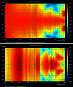
You certainly could be right about 1/3 octave smoothing being the default option when the software is first used. But it keeps your check-box selections for successive plots. Another thing that often makes a problem speaker look good is if you normalize to the on-axis response. For example, attached is a comparison of the exact same RCA data set, with normalization and heavier smoothing applied. Personally I like to see where the warts are, not hide them.Bolserst Thanks for those plots. Not as different as I expected. Perhaps the ARTA stuff that I had seen in the past was heavily smoothed by the user rather by default in the software. I would have had no way of knowing which. But I have almost never seen an ARTA map as detailed as what is shown in your left hand plot. All of the real warts are there even if they aren't exactly the same.
It would be very interesting if a speaker like this could be measured with 2deg angular increments and then compared with the results of your modal approach using the 14 angle subset of those same measurements.I think my technique works a little better near the 10 kHz point, but that is to be expected.
I also noted that in your polar map of the "good speaker" there is a ~3dB rise in response around 100Hz on-axis that is completely missing from the ARTA plot. Is this due to the LF extrapolation possible with the modal approach that you mention in your white paper?
Are your current contour lines really every 3dB?Looking at the ARTA plots, I can see that my contour lines need to be darker and perhaps more often - say 2 dB instead of 3.
After inspecting the color scale for a bit I had decided they were every 6dB.
Attachments
Exporting of multiple IR table is implemented in Arta Recorder 1.3.2. Number of samples is constant 4301. Angle is detected from the file name between "deg" and ".pir".
Bolserst
Yea normalizing and smoothing makes everything look good. One would not even know those were the same speaker.
The 3 dB "difference" between my plots and ARTA is due to the LF falling below 200 Hz from windowing in ARTA. Mine is extrapolated based on the enclosure size, driver size, f0 and Q below 200-300 Hz and matched to the monopole and dipole levels in that region. I am not exactly sure how accurate this is, except that I know it is more accurate than ARTA here because it does do anything about the windowing problem. I used to use near-field in this region, but then I found that the new technique worked just about as well.
The contour lines are every 6 dB on the web software, but I thought that they were every 3 dB on what I am using now. Some are so faint that they are hard to see. I am going to change that.
Last edited:
- Status
- Not open for further replies.
- Home
- Loudspeakers
- Multi-Way
- Measurement technology