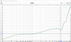
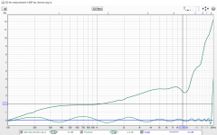
Finally, an impedance measurement with the Bode100 in series-thru mode. Measured between the two wires going from the xformers to the panels, disconnected from the xformer.
Lots of funny things seem to be going on in the upper octave!
Jan
Jan,
Here is your Bode 100 plot versus the simmed values.
Biggest difference is in the area around 20Khz.
When removing the coupling between the coils, FR at 20Khz comes much closer to your recording.
Hans
.
Attachments
Last edited:
I remember that the mutual coupling was a guesstimate only, so maybe it has to be finetuned based on the measurements.
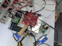
BTW Listening now to my prototype direct drive amp playing music. It is only one channel, driving one side of the panel assembly with the other side grounded, but still, sounds quite good.
Currently at a bit elevated listening level, and the signal peaks at about 1500V.
Needs some EQ because the mid/high is a bit too high wrt to the lows.
But clean, clear, very good sound.
Happy camper here!
Jan
Attachments
Last edited:
Yes, that is the equalization curve you should start with to best match the OEM acoustic response.The conclusion I draw from this is, that when I drive my direct drive amp with a flat response, the output should be equalized as in the 3rd graph.
However, you may find slight tweaks in the midrange and upper octaves improve the listening experience even further.
BTW, that now looks quite close to what I measured.
This is due to the descretization of the transmission line using lumped L & C to get delays for the different ring segments.Also interesting that the network lets go above 20 KHz.
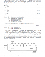
There is a cut-off frequency based on the size of the “lumps”. Attached is an excerpt from the Baxandall ESL Chapter.
Some additional details and Spice simulations provided in Post #254.
It looked like the 22Khz peak is due to the 1.5uF capacitor put across the primaries of the transformers.…the 22 KHz peak seems to be a transformer artifact, maybe to isolate the amp from the pure C load.
It didn't have any effect on the response, but did make impedance more resistive at HF. I always thought it was there to smoother out the limiter action.
Post #213
Attachments
Last edited:
The Rpar value of 300K you are using to account for damping effect of the shorted turns in the inductors is likely on the low side. Something more like 2Meg - 3Meg should provide a closer match in the upper octaves, including some of the zig-zags. I know you had set it to 300K to better match general trends of acoustic measurements, but it completely removed the ripples seen in the measurements. At that time you weren’t including any coupling between the inductors. I’m guessing some adjustment of both Rpar and the coupling coefficients would be required for best match. Unfortunately, neither is easy to measure…and there is likely additional coupling between the non-adjacent inductors.…Here is your Bode 100 plot versus the simmed values.
Biggest difference is in the area around 20Khz.
I plan to wind up some inductors this weekend that more closely match the winding geometry(ie starting from near zero radius) and see if I can get a better estimate of the coupling factors to use.
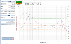
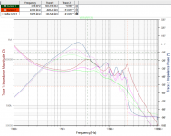
Here are the results for 1) Rpar=300K, K=0.3 and K=0.1 and 2) Rpar=2Meg, K=0.3 and K=0.1.
First image shows Jan's Bode diagram in Brown and on top of that 1) in Green and 2) in Purple.
Ripples at HF are now clearly visible as a prove that Rpar = 300K is too low when having added the coupling between the coils.
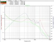
Second image shows the FR with my original live recording in Cyan, with on top 1) in Red and 2) in Blue.
Hans
.
First image shows Jan's Bode diagram in Brown and on top of that 1) in Green and 2) in Purple.
Ripples at HF are now clearly visible as a prove that Rpar = 300K is too low when having added the coupling between the coils.
Second image shows the FR with my original live recording in Cyan, with on top 1) in Red and 2) in Blue.
Hans
.
Attachments
Did some more work today towards the direct drive amp, to equalize the response to match the original speaker. Ordered a miniDSP 2x4DH as a front end, because: 1) both analog and digital inputs for experimentation, 2) provides inverted outputs to drive both panels of a speaker in opposite phase, 3) rich menu of filters and EQ.
The nice thing is that it allows calculation of filter coefficients in REW and then download those into the miniDSP.
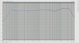
Step 1: take the xformer freq response and manipulate the data to 1) normalize at 0dBV @ 100Hz; EQ for the probe droop; invert it so that any filtering can be done by decreasing level to avoid unintended overload.
The resulting curve, loaded in REW is attachment 1. This is the inverted shape of what I posted earlier.
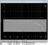
Step 2: setup REW to turn this into a flat response, normalized at 100Hz, using 8 FIR filters. The result is attachment 2. The response is flat within +/-0.2dB except at the top. I probably will roll that top of with an additional filter.
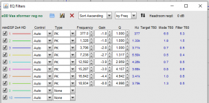
Finally, the filter settings as they need to be downloaded to the miniDSP as biquad coefficients.
All in all, not a bad result for a Sunday mornings work ;-)
Jan
PS example: 1st filter coefficients set:
biquad1,
b0=0.9974735606763722,
b1=-1.9724031392342314,
b2=0.9755301654455323,
a1=1.9724031392342314,
a2=-0.9730037261219044,
The nice thing is that it allows calculation of filter coefficients in REW and then download those into the miniDSP.
Step 1: take the xformer freq response and manipulate the data to 1) normalize at 0dBV @ 100Hz; EQ for the probe droop; invert it so that any filtering can be done by decreasing level to avoid unintended overload.
The resulting curve, loaded in REW is attachment 1. This is the inverted shape of what I posted earlier.
Step 2: setup REW to turn this into a flat response, normalized at 100Hz, using 8 FIR filters. The result is attachment 2. The response is flat within +/-0.2dB except at the top. I probably will roll that top of with an additional filter.
Finally, the filter settings as they need to be downloaded to the miniDSP as biquad coefficients.
All in all, not a bad result for a Sunday mornings work ;-)
Jan
PS example: 1st filter coefficients set:
biquad1,
b0=0.9974735606763722,
b1=-1.9724031392342314,
b2=0.9755301654455323,
a1=1.9724031392342314,
a2=-0.9730037261219044,
Attachments
Last edited:
...Step 1: take the xformer freq response and manipulate the data to 1) normalize at 0dBV @ 100Hz; EQ for the probe droop; invert it so that any filtering can be done by decreasing level to avoid unintended overload.
The resulting curve, loaded in REW is attachment 1. This is the inverted shape of what I posted earlier.
Comparing with your earlier data from Post #350, this curve doesn't match either the pre or post probe droop compensation. Any idea what the difference is?
The miniDSP 2x4HD is a great tool to work with.
It also has FIR capability if Bi-quads get too cumbersome.
Attachments
Yes there seems to be a difference. In this case, I applied the probe EQ after the measurement rather than to the source level, I have to see if that has introduced an error.
Anyway I was quite preoccupied with the whole procedure so I may have overlooked something. I will need to go through the whole thing again in detail, now I have figured out the process.
If you think about it, the tools and software we now have available to us, even not being professionals, were unheard of a couple of decades ago. And then realize that Peter Walker designed this speaker without them. Amazing.
Jan
- Home
- Loudspeakers
- Planars & Exotics
- QUAD 63 (and later) Delay Line Inductors