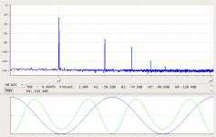
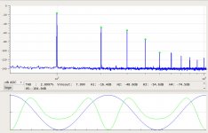
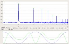
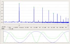
And the spectra into a 4 Ogm load at 1W, 16W, 25W, 40W, and 60W:
Attachments
-
 2SK182ESno4-2.5A-SS8R-1W-4R-spectrum.jpg100.6 KB · Views: 596
 -
 2SK182ESno4-2.5A-SS8R-16W-4R-spectrum.jpg103.7 KB · Views: 592
 -
 2SK182ESno4-2.5A-SS8R-25W-4R-spectrum.jpg101.9 KB · Views: 573
 -
 2SK182ESno4-2.5A-SS8R-40W-4R-spectrum.jpg102.8 KB · Views: 579
 -
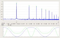 2SK182ESno4-2.5A-SS8R-60W-4R-spectrum.jpg106.8 KB · Views: 560
lhquam, I have been very interested in this thread, but I don't think I fully understand what your measurements suggest due to my very limited knowledge about electrical circuit.
I've got 2 pairs of 182ES planning to make some kind of big SE follower amp which is similar to my choke loaded Sony SIT SE follower amp currently used for compression driver, and I'm still wondering what is the best operation point for 182ES. I don't own variable power supply nor measurement tools except computer AD, so I would like to determine the power supply voltage and current/vgs before I start the test project. I wonder if you have any suggestion for me.
I've got 2 pairs of 182ES planning to make some kind of big SE follower amp which is similar to my choke loaded Sony SIT SE follower amp currently used for compression driver, and I'm still wondering what is the best operation point for 182ES. I don't own variable power supply nor measurement tools except computer AD, so I would like to determine the power supply voltage and current/vgs before I start the test project. I wonder if you have any suggestion for me.
Without any direct way to make electrical measurements, I do not know what to suggest, other than using your ear at various SIT drain voltages.
All of the 2SK128ES SITs that I have measured have the property the the required drain voltage increases with bias current and with mu-follower gain.
Vd = K*Ibias*(1+PPR)
PPR = IpullupAC/IpulldownAC. PPR=0 when the mu-follower is a constant current source.
K is approximately 3.3*RloadSS, where RloadSS is the output load impedance at the amplifier sweet-spot, which typically choose to be 6 Ohms, resulting in K=20.
The bottom line is that my samples of the 2SK182ES need a very high rail voltages to obtain high bias currents and/or high mu-follower gain factors.
With a computer sound card you can measure thd, but don't typically have an
indication of the 2nd harmonic phase. However, you can find the sweet spot where
the 2nd is at minimum. Operation at lower Vds than that gives you positive
phase 2nd, and higher gives you negative. This applies to followers.
For cases where the absolute phase is inverted (common-source mode) you
will be flipping the phase at the output, so the opposite applies.

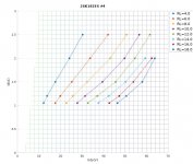
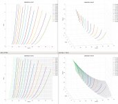
After many days of tedious measurements (and software development) I have measurements of six Tokin 2SK182ES SITs. The plots below show two different types of measurements:
Each sweet-spot curve consists of a set of measurements [Vd, Id, Vgs, RL], where RL has a constant value for the curve and the 2nd harmonic is minimum at each point.
The six 2SK182 SITs show a similar behavior for both types of measurements. As an approximation, the sweet-spot measurements show a behavior approximated by the formula:
- Vgs Curves of Id vs. Vds for constant Vgs (FrankenTracer measurements: Frankentracer Schematic | AudioMaker)
- SweetSpot Curves of Id vs. Vds for constant load impedance on SIT.
Each sweet-spot curve consists of a set of measurements [Vd, Id, Vgs, RL], where RL has a constant value for the curve and the 2nd harmonic is minimum at each point.
The six 2SK182 SITs show a similar behavior for both types of measurements. As an approximation, the sweet-spot measurements show a behavior approximated by the formula:
- Vd = 3.3*RloadSS*Id*(1+PPR)
- PPR = dI(M1)/dI(J1) is the push-pull ratio
- RloadSS is the sweet-spot output load impedance
Attachments
Design Process:
If you want the amplifier to have roughly the same harmonic constant with 4R and 8R output loads, amplifier should have a sweet-spot (2nd harmonuic minimum) near 6R (half way between 4R and 8R). This will also result in the 2nd harmonics to have opposite phases at 4R and 8R.
For an amplifier like the FirstWatt SIT-1, the SIT drain "sees" a load impedance of RL = Rload || Rdrain as shown in the 1st figure below.
For an amplifier like the FirstWatt SIT-2, SIT drain "sees" a load impedance of RL = Rload*(1+PPR), where PPR is the push-pull ratio d(I(Rhi))/d(I(Rmu)) as shown in the 2nd figure below.
The mu-follower amplifier design process is:
- Choose [Id, PPR, RloadSS]
- RL=RloadSS*(1+PPR)
- Find Vd on the RL sweetspot curve at Id.
- Id=2A, PPR=0, RloadSS=6R
- RL=6
- Result: Vd=34V
Attachments


lhquam, thank you so much for the detailed explanation.
It makes things clear, especially what I do understand now and what I still do not. It's interesting to know that 2nd harmonics to have opposite phases at 4R and 8R with 6R optimization.
Mr. Pass and Ben Mah, thank you for the information about sweet spot measurement with computer. I'm on Mac, but Wine should work.
Hi flocchini and BenMah, I already have those things. I measured my Aleph J and it worked very well. I'll try DiAna next to measure H2 phase which I have never done. Thank you!
PS: I actually measured Aleph J with RMAA, not REW. IMD can be measured, but no distortion phase.
Rightmark
PS: I actually measured Aleph J with RMAA, not REW. IMD can be measured, but no distortion phase.
Rightmark
Last edited:
I second Bob's suggestion to use REW. I used DiAna to confirm the phase, but I usually use REW to measure distortion. REW is easy to use and it displays the harmonics graphically and also numerically, making it easy to compare results.
Ben
Can I trouble you for a link/reference to DiAna? - my search engines are focussing on the Princess of Wales.
Thanks and be safe.
Bob
Thanks Dennis !!!
On first glance it appears to be a Microsoft based app - I'll explore further
Best and be safe
On first glance it appears to be a Microsoft based app - I'll explore further
Best and be safe
Exploiting the Vgs Curves
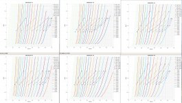
The FrankenTracer curves of Id vs. Vds for constant Vgs provide important information about the device, but in the raw form of a 2 dimensional plot if is difficult to extract that information. However it is possible to convert the 2-plot data into mathematical function of the form Vgs(Vd,Id) which can be visualized as a surface as shown in the 1st image below, showing the "raw" Vgs curves, a perspective view, and with a surface mesh of the function Vgs(Vd,Id).
I have found that the 2SK182ES Vgs surface is well approximated by the function Vgs(Vd,Id) = c1*Vd^2 + c2*Vd*Id + c3*Vd + c3*Id^2 + c5*Id + c6, where (c1,c2,c3,c4,c5,c6) are computed by least-squares fit (linear regression) to the curves samples at points (Vd, Id, Vgs). The triode parameters mu, gm, and Rdrain (Rplate) can be computed from Vgs(Vd,Id) as as shown in the 2nd image below. The 3rd image shows the least-squares solution coefficients for 2SK182ES#4 and the trioda parameters for a few values of Vd and Id.
Attachments


The FrankenTracer curves of Id vs. Vds for constant Vgs provide important information about the device, but in the raw form of a 2 dimensional plot if is difficult to extract that information. However it is possible to convert the 2-plot data into mathematical function of the form Vgs(Vd,Id) which can be visualized as a surface as shown in the 1st image below, showing the "raw" Vgs curves, a perspective view, and with a surface mesh of the function Vgs(Vd,Id).
I have found that the 2SK182ES Vgs surface is well approximated by the function Vgs(Vd,Id) = c1*Vd^2 + c2*Vd*Id + c3*Vd + c3*Id^2 + c5*Id + c6, where (c1,c2,c3,c4,c5,c6) are computed by least-squares fit (linear regression) to the curves samples at points (Vd, Id, Vgs). The triode parameters mu, gm, and Rdrain (Rplate) can be computed from Vgs(Vd,Id) as as shown in the 2nd image below. The 3rd image shows the least-squares solution coefficients for 2SK182ES#4 and the trioda parameters for a few values of Vd and Id.
Amazing work. Wow
My next challenge is to see if it is possible to obtain the sweet-spot information directly from the Vgs curves. In principal, a perfect Vgs(Vd,Id) function should contain the information for computing the nulls of the second harmonic. I suspect that the lack of precision from the 8-bit Rigol scope data capture, even after massive amounts of smoothing, might be the limiting factor.
SIT-3 Simulations
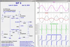
The plots below show simulations of a circuit based on the FirstWatt SIT-3 amplifier using the Tokin 2SK182ES SIT and the IXYS IXTN40P50P PFET.
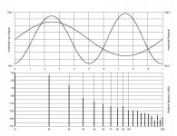
In the images shown below, the plots show the following, from top to bottom:
V(S1) Voltage at node S1.
Ix(J1:d) and Is(M1) FET push-pull currents
gmJ1 = dIJ1/dV(G1-S1) SIT J1 transconductance
RL = dV(S1)/dIJ1 Dynamic Load Resistance seen by SIT
The first image shows the simulation with Rs=1R0 and Rload=4R. Note that the the push-pull currents are nearly identical, but opposite, indicating balanced push-pull operation. The SIT transconductance is about 0.9S and the SIT sees about 8R dynamic load.
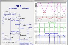
The second image shows the simulation with Rs=1R0 and Rload=8R. The SIT AC current is far below that of the PFET. The SIT transconductance is about 0.3S and the SIT sees about 32R dynamic load.
The third image shows the simulation with Rs=0R5 and Rload=8R. What gives? The SIT AC current is in phase with that of the PFET. The SIT transconductance is about -0.2S and the SIT sees about -45R dynamic load. Totally weird!
The next post with explain what is occurring.this behavior.
The plots below show simulations of a circuit based on the FirstWatt SIT-3 amplifier using the Tokin 2SK182ES SIT and the IXYS IXTN40P50P PFET.
In the images shown below, the plots show the following, from top to bottom:
V(S1) Voltage at node S1.
Ix(J1:d) and Is(M1) FET push-pull currents
gmJ1 = dIJ1/dV(G1-S1) SIT J1 transconductance
RL = dV(S1)/dIJ1 Dynamic Load Resistance seen by SIT
The first image shows the simulation with Rs=1R0 and Rload=4R. Note that the the push-pull currents are nearly identical, but opposite, indicating balanced push-pull operation. The SIT transconductance is about 0.9S and the SIT sees about 8R dynamic load.
The second image shows the simulation with Rs=1R0 and Rload=8R. The SIT AC current is far below that of the PFET. The SIT transconductance is about 0.3S and the SIT sees about 32R dynamic load.
The third image shows the simulation with Rs=0R5 and Rload=8R. What gives? The SIT AC current is in phase with that of the PFET. The SIT transconductance is about -0.2S and the SIT sees about -45R dynamic load. Totally weird!
The next post with explain what is occurring.this behavior.
Attachments

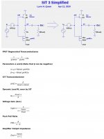
SIT-3 Circuit Analysis
I analyzed the circuit equations of a simplified version of the SIT-3 circuit. Using the the triode voltage gain formula Vgain = μ*RL/(Rdrain+RL), I obtained a simple set of circuit equations which explain the weird behavior of the circuit. The complete mathematical derivation is available upon request.
The first image below shows the simplifier circuit topology and a summary of the circuit behavior. The second image show the equations further simplified by introducing two new parameters α and β.
The weird behavior is explained by parameter β=μ-Rload*gmM1e which becomes negative when Rload*gmM1e > μ. To prevent this, PFET M1 must be degenerated by source resistor Rs. Rload can also be limited by adding a resistor in parallel with the speaker load.
Attachments

- Home
- Amplifiers
- Pass Labs
- SIT measurements, Mu Follower, and amplifier build