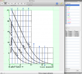
Posted a query in the other spice thread. I’m just trying to model a prospective 6AS7 amp designed by @suncalc. I couldn’t find a proper audio potentiometer model so consulted the wiki and YouTube. I came up with the attached and by luck it seems to work. I don’t know how an actual audio pot is supposed to behave and would appreciate any advice to improve it and fix errors. Thanks. https://www.diyaudio.com/forums/sof...ltxvii-beginner-advanced-259.html#post6528950
Here's the one I use.
potentiometer.asy
Code:
Version 4
SymbolType CELL
LINE Normal 32 40 32 48
LINE Normal 16 32 32 40
LINE Normal 48 16 16 32
LINE Normal 16 0 48 16
LINE Normal 48 -16 16 0
LINE Normal 32 -32 32 -24
LINE Normal 32 -24 48 -16
LINE Normal 96 16 54 16
LINE Normal 62 10 54 16
LINE Normal 62 21 54 16
WINDOW 3 -118 -22 Left 0
WINDOW 123 -60 15 Center 0
SYMATTR Value Rvalue=100
SYMATTR Value2 position=0.5
SYMATTR Prefix X
SYMATTR Description A resistor trimmer, 0<position<1
SYMATTR SpiceModel trimmer
SYMATTR ModelFile control.lib
PIN 32 -32 NONE 0
PINATTR PinName T1
PINATTR SpiceOrder 1
PIN 32 48 NONE 0
PINATTR PinName T2
PINATTR SpiceOrder 2
PIN 96 16 NONE 8
PINATTR PinName WIPER
PINATTR SpiceOrder 3
control.lib
Code:
*	-----------------------------------------------------------------------------------------------------
*	Control library for LTSpice v1.1			KM 2009
*	-----------------------------------------------------------------------------------------------------
*	The models and results are believed to be accurate, but the author cannot take any
*	responsibility for possible damage caused by mistakes or inaccuracies.
*	The content on this site is distributed in the hope that it will be useful, but WITHOUT ANY WARRANTY;
*	without even the implied warranty of MERCHANTABILITY or FITNESS FOR A PARTICULAR PURPOSE.
*
*	Use with SwitcherCAD III program, best to turn 'Skip initial operating point solution' option ON when
*	doing transient simulation.
*
*	See [url=http://home.scarlet.be/kpm/]Nap0's stuff[/url]
*	-----------------------------------------------------------------------------------------------------


*	PID controller
*	with dampened differentator for real world behavior and better convergence
*	Vo(s)/Vi(s) = Kp[ 1 + 1/(Ti.s) + Td.s/(1 + dampfactor.Td.s)]
*	parameters:
*	limit : the output is limited between +limit and -limit, the output will saturate as with real world devices
*	Kp : proportional gain constant
*	Ti : intergration time constant
*	Td : differentation time constant
*	dampfactor : higher value means more damping. When a unit step is applied to IN the differentiator term
*	will contribute a 1/dampfactor Dirac pulse to OUT
.subckt pid IN OUT GND
Gin 1 GND IN GND 1
Rp 1 2 {Kp}
Ci 2 3 {Ti/Kp}
Ld 3 GND {Kp*Td} Cpar=0
Rdamp 3 GND {1/dampfactor}
Rdummy 1 GND 1E30
Gout OUT GND 1 GND TABLE=({-limit},{-limit},{limit},{limit})
Rout OUT GND 1
.ends

*	PID controller serial implementation
*	with dampened differentator for real world behavior and better convergence
*	Vo(s)/Vi(s) = Kp[ 1 + Td.s/(1 + dampfactor.Td.s)].[1 + 1/(Ti.s)]
*	parameters:
*	limit : the output is limited between +limit and -limit, the output will saturate as with real world devices
*	Kp : proportional gain constant
*	Ti : intergration time constant
*	Td : differentation time constant
*	dampfactor : higher value means more damping. When a unit step is applied to IN the differentiator term
*	will contribute a 1/dampfactor Dirac pulse to OUT
.subckt pid_serial IN OUT GND
Gin 1 GND IN GND 1
Rp 1 2 {Kp}
Ld 2 GND {Kp*Td} Cpar=0
Rdamp 2 GND {1/dampfactor}
G1 3 GND 1 GND 1
Rp2 3 4 {Kp}
Ci 4 GND {Ti/Kp}
Rdummy 3 GND 1E30
Gout GND OUT 3 GND TABLE=({-limit},{-limit},{limit},{limit})
Rout OUT GND 1
.ends

*	subtractor
*	parameters:
*	limit : the output is limited between +limit and -limit, the output will saturate as with real world devices
.subckt sub IN+ IN- OUT GND
Gout OUT GND IN- IN+ TABLE=({-limit},{-limit},{limit},{limit})
Rout OUT GND 1
.ends

*	summator
*	parameters:
*	limit : the output is limited between +limit and -limit, the output will saturate as with
*	real world devices
.subckt sum IN1 IN2 OUT GND
Gin1 1 GND IN1 GND 1
Gin2 1 GND IN2 GND 1
Rsum 1 GND 1
Gout OUT GND 1 GND TABLE=({-limit},{-limit},{limit},{limit})
Rout OUT GND 1
.ends

*	limiter
*	parameters:
*	limit_low : the output will not go lower then limit_low, the output will saturate as with
*	real world devices
*	limit_high : the output will not go lower then limit_high, the output will saturate as with
*	real world devices
.subckt lim IN OUT GND
Gout GND OUT IN GND TABLE=({limit_low},{limit_low},{limit_high},{limit_high})
Rout OUT GND 1
.ends

*	Gain with limiter
*	parameters:
*	gain : linear gain factor
*	limit_low : the output will not go lower then limit_low, the output will saturate as with
*	real world devices
*	limit_high : the output will not go lower then limit_high, the output will saturate as with
*	real world devices
.subckt gain_lim IN OUT GND
Gin GND 1 IN GND {sgn(gain)}
Rin 1 GND 1
Gout GND OUT 1 GND TABLE=({limit_low/abs(gain)},{limit_low},{limit_high/abs(gain)},{limit_high})
Rout OUT GND 1
.ends

*	1st order phase lag
*	Vo(s)/V(I(s) = K / [1 + Tc.s]
*	parameters:
*	K : linear gain factor
*	Tc : time constant
*	limit : the output is limited between +limit and -limit, the output will saturate as with
*	real world devices
.subckt lag1 IN OUT GND
Gin 1 GND IN GND 1
R1 1 GND {K}
Ci 1 GND {Tc/K}
Gout OUT GND 1 GND TABLE=({-limit},{-limit},{limit},{limit})
Rout OUT GND 1
.ends

*	2nd order phase lag
*	Vo(s)/V(I(s) = K / [1 + 2.Damping.s/wo + (s/wo)**2 ]
*	parameters:
*	K : linear gain factor
*	wo : natural circular frequency in RAD/s
*	Damping : damping factor, value of 1 is critically damped, lower then 1 is under-damped, ..
*	limit : the output is limited between +limit and -limit, the output will saturate as with
*	real world devices
.subckt lag2 IN OUT GND
Gin 1 GND IN GND {K*1000}
Rshunt 1 GND 1m
R1 1 2 1k
L1 2 3  {1k/(2*Damping*wo)} Cpar=0 Rser=0 Rpar=1E30
C1 3 GND {2*Damping/(1k*wo)} Rser=0 Lser=0 Rpar=1E30 Cpar=0
Gout OUT GND 3 GND TABLE=({-limit},{-limit},{limit},{limit})
Rout OUT GND 1
.ends

*	absolute value
*	parameters:
*	limit : the output is limited between +limit and -limit, the output will saturate as with
*	real world devices
.subckt abs IN OUT GND
Gout GND OUT IN GND TABLE=({-limit},{limit},0,0,{limit},{limit})
Rout OUT GND 1
.ends

*	pulse width modulator
*
*	Parameters:
*	f : frequency of generated PWM signal
*	Vhigh : High level of generated PWM signal
*	Vlow : Low level of generated PWM signal
*	Range : range in which the input signal may vary, 0V gives 0% duty-cycle,
*		<Range> V gives 100% duty-cycle
*		When the input signal goes outside Range, there is no problem only the duty-cycle
*		saturates to 0% or 100%
.subckt pwm IN OUT GND
Bout GND OUT I=if(((Time-floor(Time*f)/f)*Range*f) < v(IN,GND), Vhigh, Vlow)
Rout OUT GND 1
.ends

*	pulse width modulator with complementary outputs
*
*	Parameters:
*	f : frequency of generated PWM signal
*	Vhigh : High level of generated PWM signal
*	Vlow : Low level of generated PWM signal
*	Range : range in which the input signal may vary, 0V gives 0% duty-cycle,
*		<Range> V gives 100% duty-cycle
*		When the input signal goes outside Range, there is no problem only the duty-cycle
*		saturates to 0% or 100%
.subckt pwm2 IN OUT OUTN GND GNDN
Bin GND 1 I=if(((Time-floor(Time*f)/f)*Range*f) < v(IN,GND), 1, 0)
Rin 1 GND 1
Bout GNDN OUTN I=if(absdelay(v(1,GND),deadtime)*v(1,GND) > .5, Vhigh, Vlow)
Rout GNDN OUTN 1
B2 GND 2 I=(1-v(1,GND))
R2 GND 2 1
Bout2 GND OUT I=if(absdelay(v(2,GND),deadtime)*v(2,GND) > .5, Vhigh, Vlow)
Rout2 GND OUT 1
.ends


*	SPDT switch
*	Parameters:
*	Threshold : switching level of the CONTR signal at which the switches react
.subckt spdt T1 T2 COM CONTR GND
S1 T1 COM CONTR GND swmodel1
S2 T2 COM GND CONTR swmodel2
.model swmodel1 SW(Ron=1m Roff=1000Meg Vt={Threshold} Vh=10m)
.model swmodel2 SW(Ron=1m Roff=1000Meg Vt={-Threshold} Vh=10m)
.ends

*	linear amplifier
*	Parameters:
*	gain: linear gain factor
.subckt amp IN OUT GND
Gout GND OUT IN GND {gain}
Rout OUT GND 1
.ends

*	2nd power
*	parameters:
*	limit : the output is limited between +limit and -limit, the output will saturate as with
*	real world devices
.subckt sqr IN OUT GND
Bin GND 1 I=V(IN,GND)*V(IN,GND)
Rin 1 GND 1
Gout GND OUT 1 GND TABLE=(0,0,{limit},{limit})
Rout OUT GND 1
.ends

*	square root
*	parameters:
*	limit : the output is limited between +limit and -limit, the output will saturate as with
*	real world devices
.subckt sqrt IN OUT GND
Bin GND 1 I=sqrt(V(IN,GND))
Rin 1 GND 1
Gout GND OUT 1 GND TABLE=(0,0,{limit},{limit})
Rout OUT GND 1
.ends

*	soft limiter
*	parameters:
*	limit : the output is limited between +limit and -limit, the output will saturate as with
*	real world devices
.subckt lim_soft IN OUT GND
Bout GND OUT I={limit*tanh(V(IN,GND)/scale)}
Rout OUT GND 1
.ends

*	multiplier
*	OUT = A * B in four quadrants
*	parameters:
*	limit : the output is limited between +limit and -limit, the output will saturate as with
*	real world devices
.subckt mult A B OUT GND
Bin GND 1 I=V(A,GND)*V(B,GND)
Rin 1 GND 1
Gout GND OUT 1 GND TABLE=({-limit},{-limit},{limit},{limit})
Rout OUT GND 1
.ends

*	comparator with linear zone
*	parameters:
*	linearzone : when the input is between +linearzone and -linearzone, comparator behaves linearly
*	Vhigh : High level of generated signal
*	Vlow : Low level of generated signal
.subckt comp IN+ IN- OUT GND
Gout GND OUT IN+ IN- TABLE=({-linearzone},{Vlow},{+linearzone},{Vhigh})
Rout OUT GND 1
.ends

*	integrator
*	Parameters:
*	Ti : integration time constant
.subckt int IN OUT GND
Gin GND 1 IN GND 1
Cint 1 GND {Ti}
Gout GND OUT 1 GND 1
Rout OUT GND 1
.ends

*	Dampened differentiator
*	dampened differentator for real world behavior and better convergence
*	Vo(s)/Vi(s) = Td.s/(1 + dampfactor.Td.s)
*	parameters:
*	Td : differentation time constant
*	dampfactor : higher value means more damping. When a unit step is applied to IN the differentiator term
*	will contribute a 1/dampfactor Dirac pulse to OUT
.subckt diff IN OUT GND
Gin GND 1 IN GND 1
Ldiff 1 GND {Td}
Rdamp 1 GND {1/dampfactor}
Gout GND OUT 1 GND 1
Rout OUT GND 1
.ends

*	comparator with hysteresis
*	parameters:
*	hysteresis : when the difference of the inputs reaches <hysteresis>, the output changes state
*	Vhigh : High level of output signal
*	Vlow : Low level of output signal
.subckt comphys IN+ IN- OUT GND
Bhyst IN+ A V=-hysteresis*V(1,GND)
Gin GND 1 A IN- TABLE=({-1u},-1,{+1u},1)
Rin 1 GND 1
Gout GND OUT 1 GND TABLE=({-1u},{Vlow},{+1u},{Vhigh})
Rout OUT GND 1
.ends

*	Transport lag
*	The output signal is a copy of the input signal but delayed in time by <delay> seconds
.subckt transport IN OUT GND
Gin GND 1 IN GND 2
R1 1 GND 1
T1 1 GND 2 GND Zo=1 Td={delay}
Rterm 2 GND 1
Gout GND OUT 2 GND 1
Rout OUT GND 1
.ends

*	setpoint
*	generates a constant voltage of <value> volts, alternative for the V source
.subckt const OUT GND
Iout GND OUT {value}
Rout OUT GND 1
.ends

*	unit step
.subckt ustep OUT GND
Iout GND OUT PWL(0,0,{tstep-trise/2},0,{tstep+trise/2},1)
Rout OUT GND 1
.ends

*	unit ramp
.subckt uramp OUT GND
I1 1 GND DC {slope}
C1 1 GND 1
Gout OUT GND 1 GND 1
Rout GND OUT 1
.ends

*	trimmer
*	Parameters:
*	position : wiper position between 0.0 and 1.0
*	Rvalue : total resistance value
.subckt trimmer T1 T2 WIPER
Rupper T1 WIPER {(1-position)*Rvalue+1m}
Rlower T2 WIPER {position*Rvalue+1m}
.ends

*	R-2R DAC
*	no parameters
.subckt dac OUT GND D0 D1 D2 D3 D4 D5 D6 D7
R7 D7 8 200K
R6 D6 7 200K
R5 D5 6 200K
R4 D4 5 200K
R3 D3 4 200K
R2 D2 3 200K
R1 D1 2 200K
R0 D0 1 200K
R9 8 7 100k
R10 7 6 100k
R11 6 5 100k
R12 5 4 100k
R13 4 3 100k
R14 3 2 100k
R15 2 1 100k
R16 1 0 200k
Gout GND OUT 8 0 1
Rout OUT GND 1
.ends

*	Block to measure open and closed loop gain according a proposal of Helmut Sennewald from [url=http://tech.groups.yahoo.com/group/LTspice/]404 Not Found[/url]
*	parameters:
*	OPL=1 for open loop AC simulation,
*	OPL=0 for all types of closed loop simulations
.subckt measure_loop IN OUT GND
G1 1 GND IN GND 1m
*	OPL=1 allows only DC (very very low f) to reach the output for DC operating point setting
C1 1 GND {10000*OPL + 1f}
R1 1 GND 1000
G2 OUT GND 1 GND 1
R2 OUT GND 1
I1 OUT GND AC 1 * injecting AC test signal
.ends

*	Universal adjustable voltage reference model (like the TL431)
*	parameters:
*	REF internal reference [V] (for example 2.5V)
*	GAIN gain of internal opamp [A/V]
*	CURRENT_LIM maximum current the kathode can draw [A]
.subckt universal_ref ANODE KATHODE ADJ
V1 ANODE 1 DC {REF}
G1 ANODE 2 ADJ 1 {GAIN}
R1 ANODE 2 1
G2 ANODE KATHODE ANODE 2 TABLE=(0,0,{CURRENT_LIM},{CURRENT_LIM})
.ends
Last edited:
I made a quick search but could not find the model for 6S1P triode.
It seems to be close but not the same as 6C4.
Does anybody have ?
It seems to be close but not the same as 6C4.
Does anybody have ?
I made a quick search but could not find the model for 6S1P triode.
It seems to be close but not the same as 6C4.
The 9002 is equivalent to the 6S1P (and the VT-202). Here is the Ayumi model for the 9002.
Code:
*
* Generic triode model: 9002
* Copyright 2003--2008 by Ayumi Nakabayashi, All rights reserved.
* Version 3.10, Generated on Sat Mar  8 22:42:28 2008
*            Plate
*            | Grid
*            | | Cathode
*            | | |
.SUBCKT 9002 A G K
BGG   GG   0 V=V(G,K)+0.90658712
BM1   M1   0 V=(0.01433184*(URAMP(V(A,K))+1e-10))**-0.61356953
BM2   M2   0 V=(0.70969986*(URAMP(V(GG)+URAMP(V(A,K))/20.255608)+1e-10))**2.1135695
BP    P    0 V=0.00098929697*(URAMP(V(GG)+URAMP(V(A,K))/28.541091)+1e-10)**1.5
BIK   IK   0 V=U(V(GG))*V(P)+(1-U(V(GG)))*0.00057163937*V(M1)*V(M2)
BIG   IG   0 V=0.00049464849*URAMP(V(G,K))**1.5*(URAMP(V(G,K))/(URAMP(V(A,K))+URAMP(V(G,K)))*1.2+0.4)
BIAK  A    K I=URAMP(V(IK,IG)-URAMP(V(IK,IG)-(0.00054709459*URAMP(V(A,K))**1.5)))+1e-10*V(A,K)
BIGK  G    K I=V(IG)
* CAPS
CGA   G    A 1.4p
CGK   G    K 1.2p
CAK   A    K 1.1p
.ENDSHi all,
yes I know this thread is actually about TUBE spice models...
But I guess you guys visiting this thread may also be interested in that one:
breaking news: Spicemodel for reverb tanks!
Just a hint - it is now possible to simulate reverb tanks 😀
cheers, Adrian
yes I know this thread is actually about TUBE spice models...
But I guess you guys visiting this thread may also be interested in that one:
breaking news: Spicemodel for reverb tanks!
Just a hint - it is now possible to simulate reverb tanks 😀
cheers, Adrian
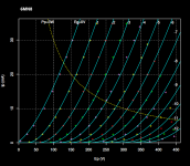
I'll try to have one for you by this evening.Does anyone have of a model for 6MN8? Thanks
6MN8 spice model
6BM8 Koren and Ayumi Nakabayashi models fresh out of the oven:
6BM8 Koren and Ayumi Nakabayashi models fresh out of the oven:
Code:
* 6MN8 LTSpice model
* Modified Koren model (6 parameters): mean fit error 0.309115mA
* Traced by Wayne Clay on Feb 23, 2021 using Engauge Digitizer 10.10
* and Curve Captor v0.9.1 from General Electric data sheet
.subckt 6MN8  P G K
    Bp  P K  I=(0.009902058429m)*uramp(V(P,K)*ln(1.0+(-0.100636358)+exp
+ ((0.7409143216)+(0.7409143216)*((104.5902961)+(-1898.200633m)*V(G,K))*
+ V(G,K)/V(P,K)))/(0.7409143216))**(1.473274341)
    Cgp G P 2.6p
    Cgk G K 4.6p
    Cpk P K 0.33p
    Rpk P K 1.0G ; to avoid floating nodes in mu-follower
    d3  G K dx1
.model dx1 d(is=1n rs=2k cjo=1pf N=1.5 tt=1n)
.ends 6MN8
Code:
*
* Generic triode model: 6MN8_AN (General Electric data sheet)
* Copyright 2003--2008 by Ayumi Nakabayashi, All rights reserved.
* Version 3.10, Generated on Tue Feb 23 19:45:32 2021
*               Plate
*               | Grid
*               | | Cathode
*               | | |
.SUBCKT 6MN8_AN A G K
BGG   GG   0 V=V(G,K)+0.18085853
BM1   M1   0 V=(0.01611335*(URAMP(V(A,K))+1e-10))**-1.2587337
BM2   M2   0 V=(0.54372773*(URAMP(V(GG)+URAMP(V(A,K))/28.316413)+1e-10))**2.7587337
BP    P    0 V=0.005418531*(URAMP(V(GG)+URAMP(V(A,K))/52.078295)+1e-10)**1.5
BIK   IK   0 V=U(V(GG))*V(P)+(1-U(V(GG)))*0.0043452991*V(M1)*V(M2)
BIG   IG   0 V=0.0027092655*URAMP(V(G,K))**1.5*(URAMP(V(G,K))/(URAMP(V(A,K))+URAMP(V(G,K)))*1.2+0.4)
BIAK  A    K I=URAMP(V(IK,IG)-URAMP(V(IK,IG)-(0.0028660811*URAMP(V(A,K))**1.5)))+1e-10*V(A,K)
BIGK  G    K I=V(IG)
* CAPS
CGA   G    A 2.6p
CGK   G    K 4.6p
CAK   A    K 0.3p
.ENDS
Attachments
You are welcome. I've noticed I wrote 6BM8 instead of 6MN8 in my post above. ^^^^ Apparently I was in a hurry. 
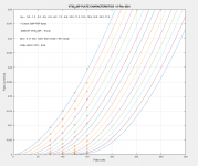
VT-20 DH triode Spice model
Hi
I have some datas about this ancient tube. 🙂 I will try some preamplifier with VT-20.
Hera are some datas: Equivalents are 220P Cossor And CV1020 tubes. I transcribe Cossor datas from Cossor 1935 PDF (very good, informative and educational...) https://frank.pocnet.net/other/Cossor/Cossor_ValveManual_1936-6.pdf
Inside is page with 220P datas.
1. Extracted data points from graph of the 220P with Graph click soft.
2. Rearanged and prepared datas for Matlab sheet (Norman Koren method)
3. I check the PSpice paramethers with Model Pain tools and etracted DHT model
4. Defined 2 pspice models, booth working with cadence orcad win soft.
cheers
Attachments
Last edited:
Does anyone have models for 6N6-G or 6B5 (dual triode with internal Loftin-White direct connection)? I've been scouring the web and can't find anything.
Hi all
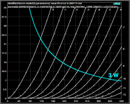
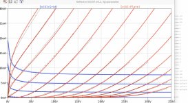
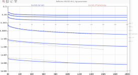
please note my latest spice model: The 6N15P!
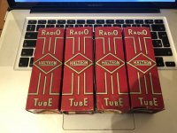
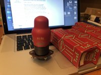
It is based on the most representative triode out of 10, after 100h burnin.
Be aware that this tube disclosed some surprisings regarding tolerances:
+ Simply the Best in terms of contact voltage
- the opposite in terms of plate resistance & grid resistance
However: If wished, plate & grid resistance may be easy adapted with the models "os" parameter to tune the model to your sample. Doubling the os value means half plate resistance.
regards, Adrian
please note my latest spice model: The 6N15P!
It is based on the most representative triode out of 10, after 100h burnin.
Be aware that this tube disclosed some surprisings regarding tolerances:
+ Simply the Best in terms of contact voltage
- the opposite in terms of plate resistance & grid resistance
However: If wished, plate & grid resistance may be easy adapted with the models "os" parameter to tune the model to your sample. Doubling the os value means half plate resistance.
regards, Adrian
Code:
*6N15P LTspice model based on the generic triode model from Adrian Immler, version i4
*A version log is at the end of this file
*100h BurnIn of 5 Reflector factory tubes, sample selection and measurements done in March 2021
*Params fitted to the measured values by Adrian Immler, March 2021
*The high fit quality is presented at adrianimmler.simplesite.com
*History's best of tube decribing art (plus some new ideas) is merged to this new approach.
*@ neg. Vg, Ia accuracy is similar to Koren models.
*@ small neg. Vg, the "Anlauf" current is considered.
*@ pos. Vg, Ig and Ia accuracy is on a unrivaled level.
*This offers new simulation possibilities like bias point setting with MOhm grid resistor,
*Audion radio circuits, low voltage amps, guitar distortion stages or pulsed stages.
*                anode (plate)
*                | grid
*                | | cathode
*                | | |
.subckt 6N15P.i4 A G K
+ params:
*Parameters for the space charge current @ Vg <= 0
+ mu   = 54    ;Determines the voltage gain @ constant Ia
+ rad  = 5k3   ;Differential anode resistance, set @ Iad and Vg=0V
+ Vct  = 0.45  ;Offsets the Ia-traces on the Va axis. Electrode material's contact potential
+ kp   = 135   ;Mimics the island effect
+ xs   = 1.50  ;Determines the curve of the Ia traces. Typically between 1.2 and 1.8
*
*Parameters for assigning the space charge current to Ia and Ig @ Vg > 0
+ kB   = 0.3   ;Describes how fast Ia drops to zero when Va approaches zero.
+ radl = 350   ;Differential resistance for the Ia emission limit @ very small Va and Vg > 0
+ tsh  = 20    ;Ia transmission sharpness from 1th to 2nd Ia area. Keep between 3 and 20. Start with 20.
+ xl   = 1.2   ;Exponent for the emission limit
*
*Parameters of the grid-cathode vacuum diode
+ kvdg  = 85   ;virtual vacuumdiode. Causes an Ia reduction @ Ig > 0.
+ kg = 470     ;Inverse scaling factor for the Va independent part of Ig (caution - interacts with xg!)
+ Vctg = -0.15 ;Offsets the log Ig-traces on the Vg axis. Electrode material's contact potential
+ xg   = 1.2   ;Determines the curve of the Ig slope versus (positive) Vg and Va >> 0
+ VT   = 0.115 ;Log(Ig) slope @ Vg<0. VT=k/q*Tk (cathodes absolute temp, typically 1150K)
+ kVT= 30m     ;Va dependant koeff. of VT
+ Vft2 = 0.5 gft2 = 10 ;finetunes the gridcurrent @ low Va and Vg near zero
*
*Parameters for the caps
+ cag  = 3p5  ;From datasheet
+ cak  = 1p85 ;From datasheet
+ cgk  = 4p4  ;From datasheet
*
*special purpose parameters
+ os = 1      ;Overall scaling factor, if a user wishes to simulate manufacturing tolerances
*
*Calculated parameters
+ Iad = {100/rad} ;Ia where the anode a.c. resistance is set according to rad.
+ ks = {pow(mu/(rad*xs*Iad**(1-1/xs)),-xs)} ;Reduces the unwished xs influence to the Ia slope
+ ksnom = {pow(mu/(rad*1.5*Iad**(1-1/1.5)),-1.5)} ;Sub-equation for calculating Vg0
+ Vg0 = {Vct + (Iad*ks)**(1/xs) - (Iad*ksnom)**(2/3)} ;Reduces the xs influence to Vct.
+ kl = {pow(1/(radl*xl*Ild**(1-1/xl)),-xl)} ;Reduces the xl influence to the Ia slope @ small Va
+ Ild = {sqrt(radl)*1m} ;Current where the Il a.c. resistance is set according to radl.
*
*Space charge current model
Bggi GGi 0 V=v(Gi,K)+Vg0 ;Effective internal grid voltage.
Bahc Ahc 0 V=uramp(v(A,K)) ;Anode voltage, hard cut to zero @ neg. value
Bst   St 0 V=uramp(max(v(GGi)+v(A,K)/(mu), v(A,K)/kp*ln(1+exp(kp*(1/mu+v(GGi)/(1+v(Ahc)))))));Steering volt.
Bs    Ai K I=os/ks*pow(v(St),xs) ;Langmuir-Childs law for the space charge current Is
*
*Anode current limit @ small Va
.func smin(z,y,k) {pow(pow(z+1f, -k)+pow(y+1f, -k), -1/k)} ;Min-function with smooth trans.
Ra  A Ai 1
Bgl Gi A I=min(i(Ra)-smin(1/kl*pow(v(Ahc),xl),i(Ra),tsh),i(Bgvd)*exp(4*v(G,K))) ;Ia emission limit
*
*Grid model
Bvdg G Gi I=1/kvdg*pwrs(v(G,Gi),1.5) ;Reduces the internal effective grid voltage when Ig rises
Rgip G Gi 1G ;avoids some warnings
Cvdg G Gi 0p1;this small cap improves convergence
.func fVT() {VT*exp(-kVT*sqrt(v(A,K)))}
.func Ivd(Vvd, kvd, xvd, VTvd)  {if(Vvd < 3, 1/kvd*pow(VTvd*xvd*ln(1+exp(Vvd/VTvd/xvd)),xvd), 1/kvd*pow(Vvd, xvd))} ;Vacuum diode function
Bgvd Gi K I=Ivd(v(G,K) + Vctg, kg/os, xg, fVT())
.func ft2() {gft2*(1-tanh(3*(v(G,K)+Vft2)))} ;Finetuning-func. improves ig-fit @ Vg near -0.5V, low Va.
Bgr Gi Ai I=ivd(v(GGi),ks/os, xs, 0.8*VT)/(1+ft2()+kB*v(Ahc));Is reflection to grid when Va approaches zero
Bs0 Ai K  I=ivd(v(GGi),ks/os, xs, 0.8*VT)/(1+ft2()) - os/ks*pow(v(GGi),xs) ;Compensates neg Ia @ small Va and Vg near zero
*
*Caps
C1 A G {cag}
C2 A K {cak}
C3 G K {cgk}
.ends
*
*Version log
*i1 :Initial version
*i2 :Pin order changed to the more common order „A G K“ (Thanks to Markus Gyger for his tip)
*i3 :bugfix of the Ivd-function: now also usable for larger Vvd
*i4: Rgi replaced by a virtual vacuum diode (better convergence). ft1 deleted (no longer needed)
;2 new prarams for Ig finetuning @ Va and Vg near zero. New overall skaling factor os for aging etc.
Attachments
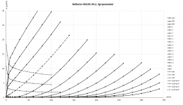
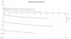
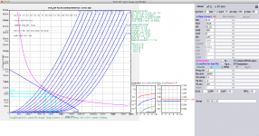
... I just realized that I posted the wrong pictures (measured curves only, but not with the model curves added)
So, here are the right diagrams, showing both, measurements and spice model curves.
regards, Adrian
So, here are the right diagrams, showing both, measurements and spice model curves.
regards, Adrian
Attachments
Hello my friends, I am studying the operation of a radio to lamps, I need in lt spice to install a library to be able to simulate a super heterodyne, for that, I need models of lamp valves type ECH81, EF85, EBC81 and the like.
The problem is that I have installed the library in LT spice and it doesn't work 🙁 I don't know what I have to do to make this library work with my program.
Can you help me how to install the library in this program so that it works correctly?
And do you have projects of super heterodynes to lamps made by you to share and thus be able to study them?
Thank you very much, have a good day.
Ayumi_LTspice
The problem is that I have installed the library in LT spice and it doesn't work 🙁 I don't know what I have to do to make this library work with my program.
Can you help me how to install the library in this program so that it works correctly?
It sounds like you might benefit from an LTspice tutorial that Mooly created in the Software Tools section of the forum. Here is a link to the first post in that thread:
Installing and using LTspice IV (now including LTXVII). From beginner to advanced.
Adding third party models to a simulation is covered in this tutorial:
Installing and using LTspice IV (now including LTXVII). From beginner to advanced.
As for the file you posted, it contains individual subcircuit files for a variety of tubes. You need to extract the models you want to use and "include" them in your .asc file as described in the second link above.
I hope this will get you started.
802 / 5000
Resultats de traducció
great, well I will review it, the question is that I could solve it, now the problem I have is knowing how I can introduce OM signal amplitude modulated AM by the input of a hectode, as well as I also need to get models of lt spice for a valve oscillating converter and I also need the detector valve models.
As a preamplifier I can use a 12ax7, but I do not have the low frequency detector diode for simulation, nor do I have the knowledge to be able to introduce the AM signal, OM amplitude modulated, and for the local oscillator valve triode I will use a 12ax7, which although it is low frequency, in LT spice I think it would work the same as the other one, joining the cathodes of the hectode with that of the triode.
I appreciate your help, have a good day.
You can find ECH81 model and its heptode.asy symbol here:
Heptode spice modelling
And I copy it here for your convenience, you can find article for Superheterodyne receiver simulation such as this one:
simulation of a superheterodyne receiver using pspice - School of ...
Most are solid state and simulation are not one complete circuit but divided sections can be simulated, RF section, Mixer, Intermediate band pass filter etc.. If you have tube circuit you can post it here see if we can simulate it.
Code:
****************************************************
.SUBCKT ECH81 1 2 3 4 5; A G3 G2G4 G1 C;
*      Extract V1.900
* Model created: 16-Mar-2014
* NOTE: LOG(x) is base e LOG or natural logarithm.
* For some Spice versions, e.g. MicroCap, this has to be changed to LN(x).
X1 1 2 3 4 5 HepthodeD MU= 47.1 MU3=    37. EX=1.448 kG1= 196.8 KP=  44.0 kVB =  2011.8 kG2= 1409.0
+ MUp=  8.5 EXX=0.518 kG1p=   5.6 KPp=3253.5 kVBp =  7766.8
+ Ookg1mOokG2=.44E-02 Aokg1=.45E-10 al=.34E-01 alkg1palskg2=.44E-02 be=  0.13 als=  5.92 RGI=2000
+ CCG1=0.0P  CCG2 = 0.0p CPG1 = 0.0p CG1G2 = 0.0p CCP=0.0P  ;
.ENDS

****************************************************
.SUBCKT HepthodeD 1 2 3 4 5; A G3 G2G4 G1 C
RE1  7 0  1MEG    ; DUMMY SO NODE 7 HAS 2 CONNECTIONS
E1 7 0 VALUE=
+{V(3,5)/KP*LOG(1+EXP(KP*(1/MU+(V(2,5)/Mu3+V(4,5))/SQRT(KVB+V(3,5)*V(3,5)))))}
E2   8 0 VALUE = {Ookg1mOokG2 + Aokg1*V(1,5) - alkg1palskg2/(1 + be*V(1,5))}
E3   9 0  VALUE = {0.5*(PWR(V(7),EX)+PWRS(V(7),EX))}
E4 10 0 VALUE=
+{V(3,5)/KPp*LOG(1+EXP(KPp*(1/MUp+V(2,5)/SQRT(KVBp+V(3,5)*V(3,5)))))}
E5   11 0  VALUE ={0.5*(PWR(V(10),EXX)+PWRS(V(10),EXX))/kg1p}
G1   1 5 VALUE = {V(8)*V(9)*V(11)}
G2   3 5 VALUE = {V(9)/kg1 *(1+Aokg1*kg1*V(1,5)- al/(1+be*V(1,5))) - V(8)*V(9)*V(11)}
RCP  1 5  1G      ; FOR CONVERGENCE    A  - C
C1   4 5  {CCG1}   ; CATHODE-GRID 1    C  - G1
C4   3 5  {CCG2}   ; CATHODE-GRID 2    C  - G2
C5   3 4  {CG1G2}   ; GRID 1 -GRID 2    G1  - G2
C2   1 4  {CPG1}  ; GRID 1-PLATE    G1 - A
C3   1 5  {CCP}   ; CATHODE-PLATE    A  - C
R1   4 15 {RGI}   ; FOR GRID CURRENT    G1 - 5
D3  15 5  DX      ; FOR GRID CURRENT    5  - C
.MODEL DX D(IS=1N RS=1 CJO=10PF TT=1N)
.ENDS HepthodeD
Attachments
- Home
- Amplifiers
- Tubes / Valves
- Vacuum Tube SPICE Models