No, I use LTSpice and stopped evaluating my designs in the 1ppm region.I understand that today we don‘t have that equipment yet.
My question was, if you perhaps came over a schematic with such ridicolous low THD numbers and possibly could point me to it ?
Thanks.

I've read the article on distortion measurements that you gave me long ago, but I'm sorry, it didn't convince me with unqualified vector errors and speed errors.
I'm not at all familiar with the algorithm you refer to, so maybe you have some paper or you could explain yourself in more detail what it does.
Generating a number of sinusoids seems easy, but what happens then, what calculations are made on those signals, the most mysterious of them is High_Y(thd(harm((v(RL)).freq).1) vs freq.
I completely fail to understand that graph.
And since I don't have Radio 2016-10, could you provide the Rogov's circuit diagram ?
Hans
Hans, to understand the essence of vector errors, I recommend that you carefully re-read the original sources again: Hafler's article, Jiri Dostal's book and an article about Bob Carver's experiment, I hope it will help.
As for the graph of THD versus frequency, I hope I explained it clearly.
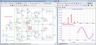
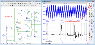
At your request, in the introduction, I added a circuit and two tests of the Rogov circuit model, where the loss of the input signal is clearly shown.
best regards
Petr
Attachments
As to the erroneous ideas of feedback 'going round and round' still turning up, despite the efforts of many smarter than me.
Look at the two inputs of the diff pair. One signal is the input, the other comes from the feedback network. Normally the second signal is phase shifted and delayed by the transit time - those are two different things. The phase shift is for audio frequencies much larger than the transit time which can be ignored for now. But there is always a continuous signal at the feedback input to the diff pair - it is not like the diff pair gets an input and then has to wait for the feedback signal!
Jan
Indeed, for periodic sinusoidal signals, the summation of phase-shifted signals gives a sinusoidal signal of exactly the same shape, but a different amplitude. Changing the phase shift changes the amplitude of the signal without affecting its shape. But this is so ONLY for sinusoidal signals.
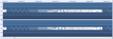
For non-stationary signals of a complex shape, such as musical signals, this is not true, for a complex signal (this is the same as for the first period of the burst of a periodic signal), there is no “tail” of the previous period for correcting the first one. We've arrived!
I am constantly remarked that signals in the form of bursts do not physically exist and it is unacceptable to use them.
Such remarks can only be made by those who are not familiar with the development of audio technology.
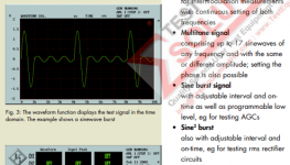
For example, the first signal in the form of bursts of frequencies from 400 Hz to 20 kHz is used to check the frequency response of the recording and playback channels of tape recorders.
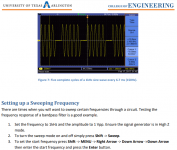
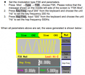
All modern generators allow you to generate any bursts, here are a few examples.
Attachments
A request to colleagues: do not litter the forum with awkward schedules, stick to the generally accepted forms of presenting information.
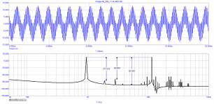
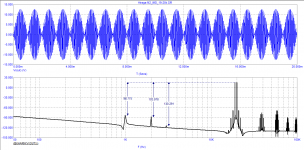
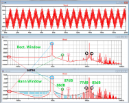
Here is an example of measuring the spectrum of harmonics at a frequency of 20 kHz of the amplifier model laid out by alnikst and examples of measuring IMD for frequencies of the same amplitude of 11.5 kHz and 950 Hz, as well as 19 and 20 kHz.
- THD in %;
- spectrum of individual signal harmonics in % or dB;
Here is an example of measuring the spectrum of harmonics at a frequency of 20 kHz of the amplifier model laid out by alnikst and examples of measuring IMD for frequencies of the same amplitude of 11.5 kHz and 950 Hz, as well as 19 and 20 kHz.
Attachments
Regarding the omnipotence of negative feedback, you can find many statements by various gurus both in textbooks and on forums. You can draw a line to this kind of statements with this post:
https://www.diyaudio.com/community/threads/sound-quality-vs-measurements.200865/post-2856456
jan, well, if you don't understand how feedback actually works, why are you putting spokes into the wheels at every step?
I have repeatedly cited statements about this by world-renowned audio developers such as Charles Hansen, Lamm, John Curl, Cyrill Hammer and many others.
Here is Nelson Pass's opinion
Audio, Distortion and Feedback
Nelson Pass
«At one extreme, the position is that “feedback makes amplifiers perfect”. At the other extreme, “feedback is a menacing succubus that sucks the life out of the music, leaving a dried husk, devoid of soul”.
Feedback is very large subject, and I am going to limit myself to some simple tutorial comments and a discussion of phenomena associated with complexity in distortion created by nonlinear gain stages, negative feedback, and the audio signal. Taken singly, these phenomena seem simple enough, but when they interact, they create distortions out of proportion to what you expect from the specifications found in product brochures.»
https://www.diyaudio.com/community/threads/sound-quality-vs-measurements.200865/post-2856456
jan.didden
«… it will always be possible engineering wise to build a 'better' amp and I expect that other measurements may be required to proof that one amp is better than another, but I have no specific answer as to which measurements this might be.»jan, well, if you don't understand how feedback actually works, why are you putting spokes into the wheels at every step?
I have repeatedly cited statements about this by world-renowned audio developers such as Charles Hansen, Lamm, John Curl, Cyrill Hammer and many others.
Here is Nelson Pass's opinion
Audio, Distortion and Feedback
Nelson Pass
«At one extreme, the position is that “feedback makes amplifiers perfect”. At the other extreme, “feedback is a menacing succubus that sucks the life out of the music, leaving a dried husk, devoid of soul”.
Feedback is very large subject, and I am going to limit myself to some simple tutorial comments and a discussion of phenomena associated with complexity in distortion created by nonlinear gain stages, negative feedback, and the audio signal. Taken singly, these phenomena seem simple enough, but when they interact, they create distortions out of proportion to what you expect from the specifications found in product brochures.»
What FFT settings are you using to get such low noisefloor?For no other reason then be able to compare LTSpice to Microsim, I simulated your circuit diagram, without knowing what Bias and what Mosfets you used.
When you want the world to follow some guidelines, let me give you some:A request to colleagues: do not litter the forum with awkward schedules, stick to the generally accepted forms of presenting information.
-IMD - in dB on a scale in a logarithmic scale.
- THD in %;
- spectrum of individual signal harmonics in % or dB;
Here is an example of measuring the spectrum of harmonics at a frequency of 20 kHz of the amplifier model laid out by alnikst and examples of measuring IMD for frequencies of the same amplitude of 11.5 kHz and 950 Hz, as well as 19 and 20 kHz.
I replicated your Hiraga circuit diagram with the 300/330R and 33/30R feedback resistors and used the same 20msec burst and a +/- 12.5V peak output.
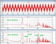
1) First thing to notice is that you apparently don't use a window, which heavily masks the image's low dB end.
Look at the example below to see the difference when using a Hann Window, where all the peaks remain the same.
2) You are showing the the distance between the signal and the 1.9Khz and 2,85Khz peaks with three decimals, however these peaks have nothing to do with IMD but are the H2 and H3 from the 950Hz signal at resp -88dB and -87dB, quite different from your figures.
3) The real IMD, 11.5Khz +/- 950Hz and 11.5Khz +/- 2*950Hz are resp at -85dB and at -77dB for IMD1 and IMD2 peaks
Staying within the 20Khz band, this results in IMD1= -82dB and IMD2= -74dB.
4) Using 3 decimals gives the impression of very accurate figures, but as has been discussed, the Microcap figures are mostly way too optimistic, where LTSpice is very close too measured results (see #1058) and therefore more reliable.
Hans
Attachments
I used a Hann Window, see posting before this one.What FFT settings are you using to get such low noisefloor?
Hans
Hans, I agree, with the Hanna window the result is more optimistic - the noise stand is significantly lower
Next, you explain common truths that do not require explanation.
best regards
Petr
Next, you explain common truths that do not require explanation.
best regards
Petr
Attachments
Last edited:
I took a deep breath and took a second look at your paper, and although I'm always in to learn new things. the scientific context of your paper don't meet the level of a simple peer review.Hans, to understand the essence of vector errors, I recommend that you carefully re-read the original sources again: Hafler's article, Jiri Dostal's book and an article about Bob Carver's experiment, I hope it will help.
As for the graph of THD versus frequency, I hope I explained it clearly.
At your request, in the introduction, I added a circuit and two tests of the Rogov circuit model, where the loss of the input signal is clearly shown.
best regards
Petr
You persist in putting forward unsubstantiated theories once formulated by some person, in many cases having a commercial agenda, and mostly on the basis of simulations that have no relation to hearing perception.
To prove any audio related theory, two things should be done:
1) doing a test with a group of people, confirming that differences can be heard when changing one single parameter and finding the threshold like for instance for Bandwidth, crossover distortion, THD, IMD or whatever.
2) the outcome of this test should be repeated and confirmed by a complete independent instance.
None of this can be found in your paper.
I copied a number of lines in your paper and gave my comment to that.
- By measuring THD with sinusoidal signals, we can only measure what the amplifier has added, but we cannot measure what it has lost.
This is a mathematical contradiction, subtraction and adding are the same process.
- Any amplifier (except the ideal one) has a limited bandwidth from above, which imposes, in addition to non-linear distortions, additional linear distortions: phase shift, change in signal amplitude.
It has been mentioned many times before: A linear system has no distortion other than graphical distortion, but not in the audio sense of THD, IMD or whatever form.
Denying this, puts all further theories on quicksand.
- Phase and gain margins often require the use of an inductor at the output of the amplifier. The presence of inductance can also be the cause of additional distortion introduced by amplifiers when operating on a real reactive load
An inductance and a resistive load form a 1th order linear filter, but you deviate from your thesis that this also distorts.
The same holds for an inductance plus capacitor forming a 2nd order linear filter that you address as being harmful, but no distortion caused by this combo.
However when the speaker forms a non linear load, the signal after the inductance might be affected, but that’s a complete different issue.
- Developers who understand the meaning of this parameter began to indicate its value in the specifications. In high quality amplifiers, this parameter rarely exceeds 100 ns! and has a constant value up to at least 300 kHz.
Show me any so called high quality amps ( to who’s standard ?) that has a constant GD up to 300Khz. If this would be so simple, why has none of the well-known manufacturers in Stereophiles A+ class this absurd BW of at least 1.6Mhz.
Because when true, that could beat the competition at arm’s length. Never asked yourself why ?
- The ear/brain is much more sensitive to time-related information than to any other parameter
Show us the prove of that, put forward as if it were a solid fact.
All well performed official tests show that at the most sensitive frequency of 3Khz, our threshold is at ca. 2msec time shift, that’s almost a phase shift of 1200 degrees !
Above 10Khz, we cannot even hear any time or phase shift.
- In analog circuits, feedback loops take a time-delayed signal from the output and send it back to the input in an attempt to correct an error that has already occurred. This creates a form of temporal distortion that cannot currently be measured, but is clearly audible.
The math (and the test equipment) tells us that the correction is fast enough, but our ears are telling us otherwise.
Just another type of distortion, temporal distortion, that apparently can’t be measured but should be heard.
This feeds the theory that feedback is bad and should be avoided.
I don’t buy this because I think that the distortion of a non-fed-back amp pleases the ears with higher even harmonics, harmonics that can be very well measured.
- Negative feedback does not work well with noise-like signals, and yet human hearing has a logarithmic dependence (Weber-Fechner law) and is very sensitive to the microlevel information of an audio signal at the noise level
Another unsubstantiated theory put forward as a fact of life.
What has noise to do with Weber-Fencher, calling this name should impress, but it is just throwing a bunch of uncorrelated things on a big heap.
- So called Vector Errors are no other than graphical differences between two signals.
Much more meaningful is using a notch filter to reveal all sorts of distortion like THD and crossover distortion.
- The assumed “Speed Errors” are also graphical differences between two signals, just showing that that the signals have differing bandwidth and or GD’s.
A Hann window has nothing to do with either optimistic nor with noise reduction. A window can't change any noise level but alters the smearing of frequencies at the cost of making the peaks BW becoming wider. So, what you indicate as noise is just spectral smearing caused by the used window.Hans, I agree, with the Hanna window the result is more optimistic - the noise stand is significantly lower
Next, you explain common truths that do not require explanation.
best regards
Petr
Sorry, but It shows a lack of fundamental knowledge on your side.
In point 1) I mentioned that all peaks remained the same after windowing, so you could have saved the time to encircle all those peaks between the two plots.
What you didn't comment are the 3 decimals with too optimistic figures, nor do you comment the fact that you ran an IMD test and measured the THD peaks instead of the IMD anomalies.
Be a man to admit when you did something wrong, that makes you a much more interesting person that is willing to learn something.
Hans
Hans, if you knew how the simulator works, you wouldn't blame me for measuring three decimal places accurately. You might think that it's my fault that the program measures with such accuracyWhat you didn't comment are the 3 decimals with too optimistic figures, nor do you comment the fact that you ran an IMD test and measured the THD peaks instead of the IMD anomalies.
Be a man to admit when you did something wrong, that makes you a much more interesting person that is willing to learn something.
don't like decimals - just drop them! 🙂
Attachments
Here are Microcap's ECW20N20/ECW20P20 models from post #1177 for LTSPice:
Microcap's mosfet parameters seem to be a mix of mosfet models. I left out all parameters not applicable to Level 1 mosfets but for some reason L & W params are needed even though they are not defined in Level 1 Mosfet.
Using these models in LTSpice IMD seems to be lower than with IRPF240/IRPF9240 but THD is much higher than in #1147. Bias resistor should be about 15ohms.
Code:
.model ecw20n20 NMOS(Level=1 Af=1 Cbd=1.95469n Cgdo=100p Cgso=100p Fc=500m Is=10f Js=10n Kp=20u Lambda=8.93602m Mj=500m Mjsw=330m N=1 Pb=800m Phi=600m Rd=272.906m Rs=124.718m TPG=1 Uo=600 Vto=-194.334m L=2u W=200.77m)

.model ecw20p20 PMOS(Level=1 Af=1 Cbd=3.08636n Cgdo=100p Cgso=100p Fc=500m Is=10f Js=10n Kp=20u Lambda=50m Mj=500m Mjsw=330m N=1 Pb=800m Phi=600m Rd=232.121m Rs=140.586m TPG=1 Uo=600 Vto=194.998m L=2u W=146.588m)Using these models in LTSpice IMD seems to be lower than with IRPF240/IRPF9240 but THD is much higher than in #1147. Bias resistor should be about 15ohms.
Best models for laterals are provided by Ian Hegglun and keantoken and are attached. I have circuit in evaluation on the bench, with Exicon 10x20 laterals (ALF08). Simulation and measured values for operating points, FR, rise time, distortion, square wave response with capacitive load …. match almost perfectly.
Attachments
In that case (ECW replaced with IRF) it might be interesting to know the quiescent current. In my sim it is 233 mA. Replacing the laterals for IRF 240 / 9240, bias set to proper value, in uC increases THD to 3.5 ppb but sim takes much longer. Will try to run, expecting IMD to be ~twice that of the laterals too.
Using Ian Hegglun's and Keantoken's models in LTSpice IMD is about the same as in #1175. With 57ohm bias resistor quiescent current is about 223mA. THD is even higher than with uCap's ECW models. LTSpice THD is about 40dB higher than in uCap so probably uCap's OPA55x model is also very optimistic. It seems uCap's distortion numbers should be taken with a large grain of salt.
Due to the difference in bias voltage, the amp's input voltage must be changed accordingly. With the IRF series I set V(in) to 9V.
Thx for making the models available.Here are Microcap's ECW20N20/ECW20P20 models from post #1177 for LTSPice:
Microcap's mosfet parameters seem to be a mix of mosfet models. I left out all parameters not applicable to Level 1 mosfets but for some reason L & W params are needed even though they are not defined in Level 1 Mosfet.Code:.model ecw20n20 NMOS(Level=1 Af=1 Cbd=1.95469n Cgdo=100p Cgso=100p Fc=500m Is=10f Js=10n Kp=20u Lambda=8.93602m Mj=500m Mjsw=330m N=1 Pb=800m Phi=600m Rd=272.906m Rs=124.718m TPG=1 Uo=600 Vto=-194.334m L=2u W=200.77m) .model ecw20p20 PMOS(Level=1 Af=1 Cbd=3.08636n Cgdo=100p Cgso=100p Fc=500m Is=10f Js=10n Kp=20u Lambda=50m Mj=500m Mjsw=330m N=1 Pb=800m Phi=600m Rd=232.121m Rs=140.586m TPG=1 Uo=600 Vto=194.998m L=2u W=146.588m)
Using these models in LTSpice IMD seems to be lower than with IRPF240/IRPF9240 but THD is much higher than in #1147. Bias resistor should be about 15ohms.
Thx, I already found Ian's models on circlotron.txt but what you just provided seems even better.Best models for laterals are provided by Ian Hegglun and keantoken and are attached. I have circuit in evaluation on the bench, with Exicon 10x20 laterals (ALF08). Simulation and measured values for operating points, FR, rise time, distortion, square wave response with capacitive load …. match almost perfectly.
Hans
- Home
- Amplifiers
- Solid State
- Musings on amp design... a thread split