Thanks for pointing this out lucky.On the contrary, if anything that's too big for that test and sample, given what we are trying to examine. IIRC 4096 was used in the 1st test, which seems sensible IMO. The samples are very analysable given standard tools and methods given what we're set to look at, and prevailing conditions. Interpretation is the issue !
I have a bit more experience working with & interpreting FFTs etc than most people.
AES E-Library Simultaneous Measurement of Impulse Response and Distortion with a Swept-Sine Technique is Prof. Angelo Farina's method for Simultaneous Measurement of Impulse Response and Distortion with a Swept-Sine Technique [2]
I worked out the theory for this circa 1990 to measure Frequency Response & THD in the theoretically shortest possible time in a noisy environment but the computing power .. and particularly good CODECs .. were far too expensive to put on every production line.
When I emerged from the bush in 2005, I found the cheapest computer had more than enough power to do this and, until recently, many good laptops like IBM/Lenovo/Apple had CODECs with textbook 16b performance. I use my 1990 method with DOS programmes and am really pleased it works as expected. 😀 The log sweep of course sounds like a B&K 2010 driven by a 2307 so must be a sweep as God intended.
I'm happy to let Angelo take credit for this as he's done far more analysis than some beach bum hu kunt reed en rite. 🙂
To add to my reply to George about RMAA, here are 5 RMAA spectrum analysis. The 20Hz - 20kHz log chirp is only 2k long but I use it with Angelo's method to make good speaker measurements in my shed .. even when the rain on the tin roof is so loud you can't hear someone next to you speak.
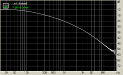
Spectrum.png is with Rectangular (no) windowing and shows the target response. Guru Wurcer will recognise the importance of slight changes in 'phase/delay' etc to allow this with 'no' windowing.
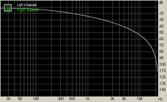
Kaiser.png is the default 2k RMAA analysis and you see it is way out.
Similarly for Hamming.png & Hanning.png BTW, the differences are way more than I'd expect with different windowing on this signal.
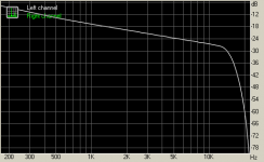
Lastly, Kaiser256.png is using 'FFT size' of 256 ie nearly 1/10 th the size of the sweep .. rather like George's measurements.
You see big differences compared to Kaiser.png and alas, the differences are at HF .. precisely the frequencies we are interested in. 🙁
So I'm not sure what RMAA is doing [1] but .. I'm sure using it to analyse a sweep much bigger than its FFT size gives nonsense at HF
And there's also the high level of 'noise' on George's sweep curves. There's something wrong if a 18s FFT type measurement has more 'noise' than a plain 'unfiltered' B&K 2307 trace.
Apologies to da Digital & Signal Processing gurus for trying to get away with some rea...aaly dodgy generalizations in the last statement 😎
The reason for trying to find the exact source of the sweep is ...
If we know this accurately enough, we can apply Angelo's method and get really supa dupa S/N & accuracy.
[1] similarly for RMAA 'Zero padding' & 'FFT overlap'
[2] available from Angelo's website
Attachments


Last edited:
This version is MUCH more stable though it still dies unexpectedly at times.
The only thing that I have found that makes RMAA 6 to die is the overdoing of expanding in the x axis. The last hit of the (+) button in the x axis makes the application to give up.
It has the large FFTs you mention.
Also you will be able to FFT files with any bit depth (while the 5.5 doesn’t accept 24bit files for FFT analysis).
I'm still wary of what it is actually doing.
eg I thought the 'FFT overlap' is 'overlap & save' processing .. a method for small computers to process large files but it isn't.
Similarly with 'Zero padding'. It's not what I thought it was
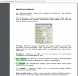
See attachment. It’s from the manual
http://audio.rightmark.org/downloads/RMAA%206.0%20User's%20Guide.pdf
George
Attachments
And there's also the high level of 'noise' on George's sweep curves. There's something wrong if a 18s FFT type measurement has more 'noise' than a plain 'unfiltered' B&K 2307 trace.
Apologies to da Digital & Signal Processing gurus for trying to get away with some rea...aaly dodgy generalizations in the last statement 😎
If you translated what the B&K is doing to a digital process, it would probably be obvious. One of the old HP spectrum analysers could be programmed to do Dick Heyser's sweep technique with a similar dramatic noise rejection.
See attachment. It’s from the manual
George
Not the most technically detailed, that's why I slog on with full math packages. One point, the FFT is inherently a linear with frequency process and most of our traditional analog way of looking at audio systems is log frequency, this might contribute to the non-intuitive better performance of short FFT's in some situations.
Not the most technically detailed,
Yes and I hope I haven't offended Ricardo.
George
Thanks George but that was the first thing I looked at.See attachment. It’s from the manual
http://audio.rightmark.org/downloads/RMAA%206.0%20User's%20Guide.pdf
I'll have to move into the 21st century and get to grips with a modern compiler or something like MathCAD or Octave.
I was bitten by MathCAD/Octave when I was pretending to be a DSP guru for AES San Francisco 2008.
That's why I like my own stuff. I think I know all the gotchas.
What is bugging me is that your 18s sweep with FFT is giving less reliable results & MUCH more noise than using a B&K 2307
0.2dB resolution with the standard 50dB pot is easily capable of showing the differences we are looking for.
Maybe I need to do a software 2307. Can't get the steam to run the real thing anymore. 😡
Should be easier to programme than a 2M FFT with my abacus. 🙂
Last edited:
That's the importance of Angelo's method. It can characterize 'weakly non-linear' systems in the shortest possible time.One point, the FFT is inherently a linear with frequency process and most of our traditional analog way of looking at audio systems is log frequency, this might contribute to the non-intuitive better performance of short FFT's in some situations.
eg it can look at high level THD in treble units with very short chirps at powers which would kill them if held for more than 1 sec. 😱
I don't think the 'short FFT' situation in RMAA is 'better' for what we are looking at. We are seeing are severe windowing effects pretending to be good measurements.
RMAA6.4.1 has saved me a lot of time confirming this.
These effects might be responsible for the 'noise' in George's pics but they DEFINITELY make nonsensical any conclusions about HF response.
"Simultaneous Measurement of Impulse Response and Distortion with a Swept-Sine Technique"
https://pdfs.semanticscholar.org/abc8/3f1297e5c033b8322f3d90d7c26423b6cc61.pdf
George
https://pdfs.semanticscholar.org/abc8/3f1297e5c033b8322f3d90d7c26423b6cc61.pdf
George
"Simultaneous Measurement of Impulse Response and Distortion with a Swept-Sine Technique"
George
Are there any appropriate test tracks on any test LP?
Richard - I slightly disagree on the comment that TDS is sensitive to "weak" non-linearity. The HP spectrum analyser I used had crystal ladder IF filters with no skirts, It is true at low frequencies some harmonics leak into the passband but in a weakly non-linear system by definition the fundamental and the rms sum of all the harmonics is virtually identical to the fundamental alone. 10% THD represents a .1db error.
By coincidence the first thing I did with the very first FFT box from Spectral Dynamics in 1981 was make chirp based acoustic radar out of ADI multipliers and other parts (just for fun).
Late edit Richard - I see now, the analog TDS does not use any digital post processing and of course there are no deconvolution artifacts.
Ricardo's concerns as expressed in this thread are found in pages 3 &4 in A. Farina's paper.
George
George
Yes I hadn't read that far and spoke too soon. Richard - could you please explain the axes on the sonographs, I'm used to them being three dimensional or with amplitude in color.
EDIT - Of course the second I take another look I see the gray scale bar on the right. This should be trivial to do in Python but I would worry at the high end that the sweeps would not be time invariant for a typical TT.
EDIT - Of course the second I take another look I see the gray scale bar on the right. This should be trivial to do in Python but I would worry at the high end that the sweeps would not be time invariant for a typical TT.
Last edited:
Happ-Shure cartridge model
I have been loaned the paper that includes the charts that Lucky put up way back at post #63. The charts are in Lawrence Happ’s 1979 paper Dynamic modelling and analysis of a phonograph stylus (JAES Vol 27, #1/2). [Thanks to the lender - you know who you are!]
Happ explains how he modelled the cartridge shank, elastomer and stylus for Shure. Shure wanted to supplement their first-order electrical analog models with a higher-order mechanical model to explore questions like:
The Happ-Shure model is a hands-on “what if?” tool for mechanical engineers. It includes a flexible shank, terminated at one end in a transducer (the magnet) on a pivot and, on the other end, a stylus riding on vinyl. Happ walks through the progressive development of the model. It starts simple then expands to include damping and elasticity at both the pivot and the stylus. The elastic and damping parameters at both points were determined experimentally. They needed to be included to produce results that were in good agreement with the measured response of the real system.
For the simplest of the Happ-Shure models, first resonance was at 19.5kHz with the second at 35kHz. These results are consistent with 1) the pivot including both elasticity and damping courtesy of the elastomer grommet or “rubber bung” (ie: the shank is not a “pure”, clamped cantilever), and 2) compliance and damping from the vinyl. Happ explains how both conditions were necessary for the model to produce good results.
Shure’s online technical seminar shows that this sort of modelling was used to develop cartridges including the V15-IV and V. It seems likely that other manufacturers use(d) similar tools, especially now that computing power is cheap.
It’s a good paper. In my view, it's worth the price of the AES download, though it's a shame it's not freely available.
I have been loaned the paper that includes the charts that Lucky put up way back at post #63. The charts are in Lawrence Happ’s 1979 paper Dynamic modelling and analysis of a phonograph stylus (JAES Vol 27, #1/2). [Thanks to the lender - you know who you are!]
Happ explains how he modelled the cartridge shank, elastomer and stylus for Shure. Shure wanted to supplement their first-order electrical analog models with a higher-order mechanical model to explore questions like:
What is the effect on response and trackability of increasing the [shank] wall thickness from 0.025mm to 0.038mm? (page 3)
The Happ-Shure model is a hands-on “what if?” tool for mechanical engineers. It includes a flexible shank, terminated at one end in a transducer (the magnet) on a pivot and, on the other end, a stylus riding on vinyl. Happ walks through the progressive development of the model. It starts simple then expands to include damping and elasticity at both the pivot and the stylus. The elastic and damping parameters at both points were determined experimentally. They needed to be included to produce results that were in good agreement with the measured response of the real system.
For the simplest of the Happ-Shure models, first resonance was at 19.5kHz with the second at 35kHz. These results are consistent with 1) the pivot including both elasticity and damping courtesy of the elastomer grommet or “rubber bung” (ie: the shank is not a “pure”, clamped cantilever), and 2) compliance and damping from the vinyl. Happ explains how both conditions were necessary for the model to produce good results.
Shure’s online technical seminar shows that this sort of modelling was used to develop cartridges including the V15-IV and V. It seems likely that other manufacturers use(d) similar tools, especially now that computing power is cheap.
It’s a good paper. In my view, it's worth the price of the AES download, though it's a shame it's not freely available.
Regarding Ricardo’s answer here
http://www.diyaudio.com/forums/analogue-source/303389-mechanical-resonance-mms-92.html#post5090047
Let’s say that an engineer feeds a flat 20Hz-20KHz log sweep into an electrodynamic cutter head, then cuts a track and that track is read by an electrodynamic cartridge and amplified flat.
What will be the wave envelope and the FFT of the initially flat signal which has passed through two velocity-responding transducers?
A hand drawing will greatly help.
George
Regarding Ricardo’s answer here
http://www.diyaudio.com/forums/analogue-source/303389-mechanical-resonance-mms-92.html#post5090047
Any real math package is solely limited by memory size or maybe 32 vs. 64bit. IIRC there used to be a max size for .wav or mp3 files.
Last edited:
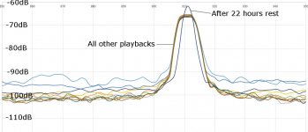
Those diagrams showed that while the 300Hz fundamental remained at the same level btn the 1st playback and +22hour playback, the harmonics haven’t.
I think what we are looking for is easy to see using any reasonable FFT method.......
Concerning the 300Hz tone tests, George posted consistently recorded samples of 10 consecutive recordings without rest time, and one recording after 22 hours.
I've now had time to look at these, and here's my 2p worth of interpretation:
The +22hr recording is distinct from the other 10 as to cart-arm low frequency resonance spectrum, which are otherwise all similar. The +22 hr sample is significantly suppressed in amplitude of the cart-arm resonant system, perhaps 3-6dB overall.
This correlates with improved FM stability for the 300Hz test tone in the +22hr sample versus all other recordings which are similar. This is confirmed by improved FM stability in all harmonics of the test tone in the +22hr sample: the peaks are sharper versus all other recordings, and this effect progresses with higher harmonic orders as expected.
Consequently, although peak levels of the test tone/harmonics are generally notably higher for the +22hr sample, eg c +6dB for 3rd harmonic peak level, this is really an artefact of a sharper peak rather than more spectral energy in the harmonic.
Attached is a plot which shows this for the 3rd harmonic, though the test tone and all other harmonics follow the same pattern to and extent that progresses with increasing harmonic order, as expected.
IMO, any differences in peak level of harmonic distortion in the +22hr sample are dominated by expected artefacts of improved FM modulation, probably arising from improved headshell lf stability.
A very interesting question is why was the +22hr sample more lf stable than the 1st sample, which presumably was also recorded after a long rest ? (George, can you please confirm the 1st sample recording was also made after a long rest ?)
A distinct feature of the 1st sample is that the noise floor is significantly adverse, perhaps c 6dB or so. Whereas there is some variance between all other recordings, including the +22hr sample, the 1st sample is quite separate.
So I think there are two confident differences observable from George's test: a) improvement in low frequency stability after 22 hours rest and b) adverse noise floor in the 1st sample recording.
OK, so now perhaps it's a case of head scratching to try to work out physically what might be going on as to a cause........... which might be experimental or might be real I suppose ?!
LD
Attachments
Last edited:
I don't design cutter heads ... but if we are talking about something that a mastering engineer would call "without RIAA pre-emphasis" ...Let’s say that an engineer feeds a flat 20Hz-20KHz log sweep into an electrodynamic cutter head, then cuts a track and that track is read by an electrodynamic cartridge and amplified flat.
What will be the wave envelope and the FFT of the initially flat signal which has passed through two velocity-responding transducers?
The Wave Envelope would be 'flat' with the addition of
- the arm/cartridge resonance/HP filter
and
- HF effects due to loading
The FFT would look like spectrum.png, the 1st pic in #921 With an 18s sweep, the Gibbs type effects at HF would be 'less' and the -3dB/8ve line would extend closer to 20Hz at LF.
That's assuming a 2M FFT or bigger to include the 1M8 recording and 'proper' zero padding to allow for the larger FFT size and any windowing
A smaller FFT with a proper 'overlap & save' scheme may not show the LF response peaks but should be OK at HF.
__________________
That was my starting point in 1990. There were proposed TDS instruments based on AD 4 quadrant multipliers & swept bucket brigade filters before that for factory test.One of the old HP spectrum analysers could be programmed to do Dick Heyser's sweep technique with a similar dramatic noise rejection.
The B&K 2010 could be a TDS instrument and we were Beta testers for most new B&K stuff at that time. The 2010 with 1902 was also B&K's THD instrument for a looo.oong time.
The log sweep was to improve S/N. My idea was to use simultaneous sliding digital filters to pick up fundamental and each harmonic from each digitally measured sweep.
The 'bingo' moment was the realisation that just de-convolving the log chirp with the received signal did this automatically and brought out the harmonics as separate 'impulses'.
At first I wanted fancier 'filters' but the matched filter provided by the log sweep which has sorta a sinc shape is so narrow (1/18s = 0.055Hz) that this has never been a practical problem .. even with the short log chirps I'm forced to use with my Jurassic software.
Sorry for the above wanking. What I wanted to say was ...
_______________
If you pretend one of Georges 18s sweeps is an impulse, you can apply Heyser's ETC processing which would give you the magnitude of his 'analytic' .. in effect doing synchronous rectification.
You can take this ETC with its
- dB y-axis
and
- rename the 18 second time x-axis "20Hz - 20kHz".
This would give you a 'real' B&K 2307 type curve with very fast writing speed. A little averaging in dB would give exact 2307 writing speed emulation. 😱
Alas, I'd need the 2M FFTs to do this in Cooktown. 🙁
BTW, I think Heyser's TDS paper is the only one which shouldn't be consigned to the Don't Recycle Bin. The others were obfuscating bullsh*t. It took me nearly 2 decades to realise this.
Last edited:
"Simultaneous Measurement of Impulse Response and Distortion with a Swept-Sine Technique"
Len Gregory has just told me the 'engineer' who provided the sweep for HFN002 has retired & become a beach bum. Has lost touch with him for years 😡
Any 'good' log sweep can be used .. provided we have an 'accurate' copy of the original.Are there any appropriate test tracks on any test LP?
Len Gregory has just told me the 'engineer' who provided the sweep for HFN002 has retired & become a beach bum. Has lost touch with him for years 😡
Thanks Bondini, and I agree it is still the best treatment of the topic available AFAIK.The Happ-Shure model is a hands-on “what if?” tool for mechanical engineers. It includes a flexible shank, terminated at one end in a transducer (the magnet) on a pivot and, on the other end, a stylus riding on vinyl. Happ walks through the progressive development of the model. It starts simple then expands to include damping and elasticity at both the pivot and the stylus. The elastic and damping parameters at both points were determined experimentally. They needed to be included to produce results that were in good agreement with the measured response of the real system.
For the simplest of the Happ-Shure models, first resonance was at 19.5kHz with the second at 35kHz. These results are consistent with 1) the pivot including both elasticity and damping courtesy of the elastomer grommet or “rubber bung” (ie: the shank is not a “pure”, clamped cantilever), and 2) compliance and damping from the vinyl. Happ explains how both conditions were necessary for the model to produce good results.
The principle point, IMO, is that cantilever self-flex is the primary element that moves in the model: the resonances at 19.5kHz and 35kHz are modes of cantilever flex resonance, rather than rigid body mass-spring with either the suspension end or the vinyl contact end. Though these ends set boundary conditions and therefore can modify the resonance in principle.
The author doesn't disclose any detail or values about boundary conditions, not even their relative magnitudes. He discusses characterising spring and damping for the suspension end, but there's no mention of the vinyl end. The only mention vinyl compliance gets is in an 'industry standard' conversion of trackability displacement to impedance, which conversion is based on a flawed assumption of what flexes, I suggest.
In the examples shown of normal cantilever modal resonances, both vinyl end and suspension ends are free pivots, otherwise not moving, ie not requiring displacement or a free end. It's the nature of impedance to rotation at each end that is at issue, IMO. There's nothing in there that contradicts vinyl compliance being far lower than that of the cantilever, and nothing that requires vinyl deformation.
Back to the OP, the 1979 Happ paper confirms there can be significant phase shift between stylus and generator ends of a cantilever: 90deg@19.5kHz, 180deg@35kHz are examples. This is not a minimum phase system, and when it comes to accurate digital correction, such group delay needs to be properly modelled if one is to be strict. This is something that would be difficult, to say the least, to implement in analog electronics, and AFAIK has never been accurately done.
So there's a fresh opportunity for the DSPmeisters.........(!)
Thanks for an interesting post, Bondini.
LD
Last edited:
A very interesting question is why was the +22hr sample more lf stable than the 1st sample, which presumably was also recorded after a long rest ? (George, can you please confirm the 1st sample recording was also made after a long rest ?)
Thanks Lucky for taking the time to work on those files.
Now regarding your question about the long rest.
As I have mentioned, before the 1st playback as well as before the after 22h playback, I exercised the cartridge by playing for 20 minutes a musical record.
So it is only the 300Hz track of the HFN test LP (and not the cartridge/headshell) which had a long rest before the 1st play back and before the +22 hours playback.
And this was intentional, as what I wanted to test with these recordings is the behavior of vinyl only (what Ricardo has mentioned) i.e.
a) that vinyl playback is not the same btn 1st and second play of the same track
b) vinyl needs a lot of time to recover after the 1st play (he mentioned 24 hours).
The hypothesis of vinyl relaxation time is to be tested more methodically in the second run of recordings (this with the 2.5gr VTF, see post # 918 for uploaded links) where after the repeated 10 playbacks each 30 sec apart, I do subsequent playbacks after 15 minutes, then after 30 minutes from the previous, then after 1 hour, 2 hours, 4 hours, 8 hours and 16 hours.
Before the 1st play and every delayed replay after the 10th, I played for 15min the same musical record. I placed (stacked) the musical record on top of the HFN test LP, so in all these recordings the HFN test LP remained in the platter unmoved.
In the first run (1.6gr VTF) and in the second run (2.5gr VTF) the same setup was used (test track, TT/platter mat/tonearm, headshell, cartridge (Stanton MKV D5), wiring, preamplifier, soundcart, PC notebook, recording SW).
These days I will conduct a third run (1KHz track from another test LP, another headshell and Shure M97xE cartridge.
George
- Home
- Source & Line
- Analogue Source
- mechanical resonance in MMs