
@keantoken: ... Wow, thank you very much for such an elaborate reply ;-) I look forward to look further into it ... it will probably be tomorrow ...
Cheers & thanks again,
Jesper
Cheers & thanks again,
Jesper
Hi all,
... I am still interested in simulating the output noise & output impedance of e.g. the CCSes found in #1635 (the collector & drain noise & output impedances) - so if one of you has some insights in this I'd appreciate your feedbacks ...
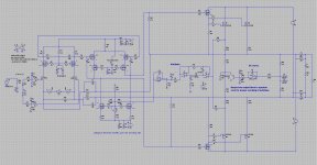
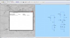
@keantoken: Thanks again for your elaborate feedback and suggestions in #1639 ... I've tried to simulate the two circuitries that can be seen in attachment #1 using your suggestions, however, I get some somewhat peculiar results. I wonder what may cause this - maybe I can ask you to clarify?
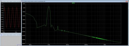
I have done this for both the second circuitry and the first NJFET based circuitry. As can be seen in the first attachment I get quite similar output impedance values ~ 102 kohms ~ for both circuitries. This in itself is a bit surprising as I would have expected the second circuitry to have a somewhat higher output impedance that the NJFET circuitry. Also, I would have expected the impedances to be higher than they are 😕 ... And there is no phase curve either ...
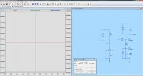
In order to try to verify the value the entered expressions give, I have measured the currents passing through J3 and Q2 and then replaced the two 10VDC voltage sources with two current sources outputting the respective currents. Thus the output impedance of J3 and Q2 would be a parallel connection between the 10e17 ohms output impedance of the current sources and either J3's drain or Q2's collector. I don't know if this works, though 🙄 (it will also only be a DC impedance/resistance) ... one indicator that it may not is that the impedances found with a transfer function calculation is quite high (the last two attachments show this).
Any chance I can ask you to verify that the expression you suggested (V(Iout2,Vneg)/Ic(Q1)) is correct?
I've also looked into LTspice's help file (viewer overview -> waveform arithmetic) and it seems to me that what is described there is more of a "general" or "overview" character. I admittedly learn best seeing examples such as e.g. your expression above ...
Regarding your capacitance & inductance real & imaginary examples I will keep them in mind should they at some point in time be needed ... right now I'd appreciate help with the noise & impedance expressions 😉
Cheers,
Jesper
... I am still interested in simulating the output noise & output impedance of e.g. the CCSes found in #1635 (the collector & drain noise & output impedances) - so if one of you has some insights in this I'd appreciate your feedbacks ...
@keantoken: Thanks again for your elaborate feedback and suggestions in #1639 ... I've tried to simulate the two circuitries that can be seen in attachment #1 using your suggestions, however, I get some somewhat peculiar results. I wonder what may cause this - maybe I can ask you to clarify?
To directly plot the impedance of the second circuit you would right click on a trace name in the waveform viewer and enter this:
V(Iout2,Vneg)/Ic(Q1)
You will get a phase and magnitude plot. If you right click on the magnitude scale, you can change between Bode, Cartesian and Nyquist coordinates.
I have done this for both the second circuitry and the first NJFET based circuitry. As can be seen in the first attachment I get quite similar output impedance values ~ 102 kohms ~ for both circuitries. This in itself is a bit surprising as I would have expected the second circuitry to have a somewhat higher output impedance that the NJFET circuitry. Also, I would have expected the impedances to be higher than they are 😕 ... And there is no phase curve either ...
In order to try to verify the value the entered expressions give, I have measured the currents passing through J3 and Q2 and then replaced the two 10VDC voltage sources with two current sources outputting the respective currents. Thus the output impedance of J3 and Q2 would be a parallel connection between the 10e17 ohms output impedance of the current sources and either J3's drain or Q2's collector. I don't know if this works, though 🙄 (it will also only be a DC impedance/resistance) ... one indicator that it may not is that the impedances found with a transfer function calculation is quite high (the last two attachments show this).
Any chance I can ask you to verify that the expression you suggested (V(Iout2,Vneg)/Ic(Q1)) is correct?
I've also looked into LTspice's help file (viewer overview -> waveform arithmetic) and it seems to me that what is described there is more of a "general" or "overview" character. I admittedly learn best seeing examples such as e.g. your expression above ...
Regarding your capacitance & inductance real & imaginary examples I will keep them in mind should they at some point in time be needed ... right now I'd appreciate help with the noise & impedance expressions 😉
Cheers,
Jesper
Attachments
EDIT, sorry that was totally wrong. You are in transient analysis, you need to go to AC analysis. Comment out the .tran command with ctrl-rightclick, click run and fill out the AC tab.
Last edited:
Thanks for a great thread. I have looked hard to find how to do a TIAN probe usage, but have not been able to find any coverage, would someone direct me to it Please. Thanks
Tian Probe
LTspice has a good example for how to perform a Tian probe. Look in the "Educational" folder under the "examples" folder for a file named LoopGain2.asc. This should get you started.
LTspice has a good example for how to perform a Tian probe. Look in the "Educational" folder under the "examples" folder for a file named LoopGain2.asc. This should get you started.
@keantoken:
Well, that is what happens - thanks for updating ... I have tried your AC analysis suggestion and it seems to work ... I do get some odd results now and then, though - might just need getting used to using this functionality ...
Cheers,
Jesper
EDIT, sorry that was totally wrong. You are in transient analysis, you need to go to AC analysis. Comment out the .tran command with ctrl-rightclick, click run and fill out the AC tab.
Well, that is what happens - thanks for updating ... I have tried your AC analysis suggestion and it seems to work ... I do get some odd results now and then, though - might just need getting used to using this functionality ...
Cheers,
Jesper
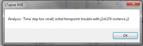
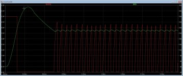
I do not understand, I had this schematic working fine in the old ltspice, and now I did it again and it does not work anymore, and I have who do not work now.
is this because of the 64 bit version? or do i miss something.
the pic you see it working in the 32 bit times.
regards
is this because of the 64 bit version? or do i miss something.
the pic you see it working in the 32 bit times.
regards
Attachments
referring to post # 19 I was playing around with variables but they seem to slow sim down quite a bit. here's what I cam up with
.tran 0 {c/f} {(c/f)-(80/f)} {(20/f)/262144}
.param f 4000
.param c 1000
and
SINE(0 0.1 {f} 0 0 0 {c}
Is there a better way?
.tran 0 {c/f} {(c/f)-(80/f)} {(20/f)/262144}
.param f 4000
.param c 1000
and
SINE(0 0.1 {f} 0 0 0 {c}
Is there a better way?
Attachments
As far as I know, this calculation for the replaceable parameter values is done once, at the startt of the sim. So it's hard to see how this can slow it down.
OTOH, you may have come up with specific numbers that cause more iterations (like smaller timesteps, not automagically adapting to voltage/current step changes) that could cause longer sim times.
Jan
OTOH, you may have come up with specific numbers that cause more iterations (like smaller timesteps, not automagically adapting to voltage/current step changes) that could cause longer sim times.
Jan
Thanks Jan. Here's another iteration. It was probably increasing the coupling caps to 1F
These should be calculated before the sim as well?
text description: ct = cycle total cs = cycles to sample
SINE(0 0.1 {f} 0 0 0 {ct})
.tran 0 {ct/f} {(ct/f)-(cs/f)} {(20/f)/262144}
.options plotwinsize=0
.param f 4000
.param ct 1000
.param cs 80
These should be calculated before the sim as well?
text description: ct = cycle total cs = cycles to sample
SINE(0 0.1 {f} 0 0 0 {ct})
.tran 0 {ct/f} {(ct/f)-(cs/f)} {(20/f)/262144}
.options plotwinsize=0
.param f 4000
.param ct 1000
.param cs 80
Attachments

I got caught with this one in the past.
1F doesn't equal what you think it equals 😉
1R is 1 ohm
1H is 1 Henry
1F is very very very tiny (Femto). Just use 1 for 1 Farad.
1F doesn't equal what you think it equals 😉
1R is 1 ohm
1H is 1 Henry
1F is very very very tiny (Femto). Just use 1 for 1 Farad.
Thanks Mooly, I was talking English there, but good to know.
Mathi is fun I see 262144 is 512 squared but not sure what the constant is
What is 2**19 ?
Mathi is fun I see 262144 is 512 squared but not sure what the constant is
What is 2**19 ?
It's all powers of two. The more, the more resolution. 2**19 or 2^19 is 2 * 262144 which is 524288.
512 is 2^9 (As we all know, 1024 is 10 bits is 2^10. 512 is half of that so 9 bits ;-)
So 512 squared = 512^2 is 9 + 9 = 18 bits.
And so on. It pays to be familiar with it.
Jan
512 is 2^9 (As we all know, 1024 is 10 bits is 2^10. 512 is half of that so 9 bits ;-)
So 512 squared = 512^2 is 9 + 9 = 18 bits.
And so on. It pays to be familiar with it.
Jan
Maths was a subject I always struggled with (big time) I'm afraid.
** I've no idea what that means as written (honest 🙂) and neither does a 5 minute web search on mathematical symbolusage turn anything up for me for that one.
All I found was:
Exponentiation in Python - should I prefer ** operator instead of math.pow and math.sqrt? - Stack Overflow
The constant thing as you ask it is another mystery (to me). No idea what you mean.
🙂
Edit... thank you Jan
As far as I know, this calculation for the replaceable parameter values is done once, at the startt of the sim. So it's hard to see how this can slow it down.
OTOH, you may have come up with specific numbers that cause more iterations (like smaller timesteps, not automagically adapting to voltage/current step changes) that could cause longer sim times.
Jan
This is what I use.
Your process probably easier.
Jan
Indeed smaller step time makes simulation longer , i have no idea how Spice really works, but i will use your idea too and compare with Mooly's solutions in post 19 which i never used until last week.It does make sim time longer what Mooly suggested , but the results are indeed more resolute.What i saw though was that the LtSpice compression function and higher step time aren't really a bad thing, it actually give very predictable results and saves time .
It's just that other people like to see some high resolution pictures when investigating other people's work.
When you're making 100 simulations in a raw, the lower resolution isn't something wrong.You'll get the same results anyway just faster.
Exponentiation (raise to the power of ..) is sometimes written as A ^^ B (A to the power of B); the logic is that * is multiplication and ** is a step up as it were.
It depends a bit on what characters are allowed in a specific app and/or the language parser rules, whether you'd use A^B or A**B but they mean the same.
Not sure what you are referring to here?
Jan
It depends a bit on what characters are allowed in a specific app and/or the language parser rules, whether you'd use A^B or A**B but they mean the same.
The constant thing as you ask it is another mystery (to me). No idea what you mean.
Not sure what you are referring to here?
Jan
- Home
- Design & Build
- Software Tools
- Installing and using LTspice IV (now including LTXVII), From beginner to advanced