@George: If you are able to get a good measurement of L and R for those Ortofons you have I would be most appreciative.
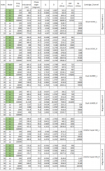
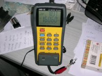
Bill, here are what I’ve measured with a DER EE LCR meter DE-5000 (it’s the same with the IET DE-5000)
https://www.ietlabs.com/pdf/Manuals/DE_5000_im.pdf
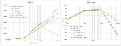
For completeness, in tabulated form are the Rs and the Rp mode measurements. The diagrams are based on the series mode measurements.
Published data for the three cartridges are as follows:
Shure M97xE: Inductance: 650mH, DC Resistance: 1550 Ohm
Dual DN165E: Inductance: 450mH, DC Resistance: 750 Ohm
Ortofon Super OM10: Inductance: 580mH, DC Resistance: 1000 Ohm
DE-5000 outputs a sinusoidal signal 0.5-0.7VRMS at the impedance range of these carts
Days later I will finish the frequency sweep impedance measurement on the same cartridges with lower excitation and will post results.
George
Attachments

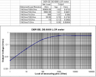
That LCR meter looks to have a source resistance around 200R, so this might limit its accuracy above about 2k impedance
David
I have provided the link to the manual. Please take a look at pages 39, 40 (Accuracy specifications) of the manual.
Accuracy is good when the open-short cal is performed.
The problem is that at 100kHz cartridge core losses affect measurements a lot.
In the previous cartridge set measurements I had done, voltage-current method (up to 20kHz) was in agreement with the LCR measurements at the four frequencies (up to the 10kHz)
George
Attachments
George,
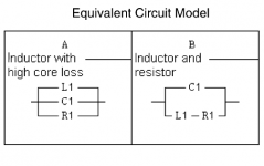
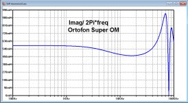
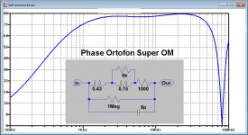
To further test a Spice model in more depth, a model that I made some time ago, I selected and simulated your Ortofon Super OM.
After some fiddling, the phase and the inductance that you found are corresponding with my model up to 10kHz.
There was no data past 10kHz, so I guessed a bit.
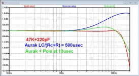
With this Calculated Cart I have simulated FR through a voltage and a current Preamp.
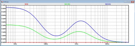
The optimum termination for a voltage amp was 47K//220pF, see red line below. Here you also see the dent in the FR between 2Khz and 10kHz, that Scott and others experienced.
For a virtual gnd amp like the Aurak, see FR in blue, you will have to compensate with an extra pole because of the Cart’s split coil.
In this case I have taken a 10usec Pole, result in green.
This all is of course with the restriction that my Cart model is correct.
Hans
To further test a Spice model in more depth, a model that I made some time ago, I selected and simulated your Ortofon Super OM.
After some fiddling, the phase and the inductance that you found are corresponding with my model up to 10kHz.
There was no data past 10kHz, so I guessed a bit.
With this Calculated Cart I have simulated FR through a voltage and a current Preamp.
The optimum termination for a voltage amp was 47K//220pF, see red line below. Here you also see the dent in the FR between 2Khz and 10kHz, that Scott and others experienced.
For a virtual gnd amp like the Aurak, see FR in blue, you will have to compensate with an extra pole because of the Cart’s split coil.
In this case I have taken a 10usec Pole, result in green.
This all is of course with the restriction that my Cart model is correct.
Hans
Attachments
Interesting, so are you saying the split pole will behave differently from solid? Note the Dual cartridge George measured is an OM (solid pin) as per the Aurak FR measurements LD has posted before.
Since I only have data up to 10kHz, the FR part from 10kHz up to 20kHz is less reliable, but keep in mind that also LD had to insert an extra pole, in his case 3.3usec.Interesting, so are you saying the split pole will behave differently from solid? Note the Dual cartridge George measured is an OM (solid pin) as per the Aurak FR measurements LD has posted before.
Unfortunately Georges LC meter has no frequency between 10kHz and 100kHz, and at 100khz there may be no measurement possible ?
Hans
P.S. The morale is quite simple, the more points there are available, the more accurate the model.
Last edited:
I am having a dim day. Surely a 3.3us pole is just to roll off ultrasonics and maintain stability?. It really wont change things much below 20kHz?
Yes it does below 20kHz, have a look atI am having a dim day. Surely a 3.3us pole is just to roll off ultrasonics and maintain stability?. It really wont change things much below 20kHz?
Cartridge dynamic behaviour
Here you see the same uplift, that was only mildly suppressed by 3.5usec,
Red versus blue line.
I went a bit further with 10usec in suppressing the peak.
But again, my model could use a number of extra measurement.
Ideal would be the outcome of an A/R vector analyzer.
Hans
Ah yes I see. The scaling had thrown me. Given Ortofon voice their MCs for a 2dB lift at 20kHz this could almost be seen as a benefit!
I'd personally rather dial in a gentle shelf to correct up to 20kHz but I do have DSP spare and am a heretic in the eyes of some 🙂
I'd personally rather dial in a gentle shelf to correct up to 20kHz but I do have DSP spare and am a heretic in the eyes of some 🙂
To complete the measurements taken from the Adjust+ record, played at 3 different speeds, I produced the images below.
The relevant images are unprocessed and recorded under exactly the same conditions.
One big difference is that the PN on the Adjust+ covers more than 4 decades, from 5Hz to 20kHz, versus slightly more than a decade from 2Khz to 30kHz for the CH Precision.
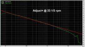
So playing the Adjust+ with its wide bandwidth at resp 33 1/3, 45 and 60.75rpm, causes quite some deviation from the ideal -10dB/oct PN roll off.
That's because at different speeds pre-emphasis on the record is no longer matched with the Riaa de-emphasis.
This is shown in the first image below.
At 33 1/3 rpm everything is o.k. resulting in the straight red line.
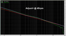
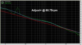
At 45rpm the deviation is shown with the green line and for 60.75rpm the blue line.
That's what I have visualised in the images below.
The red line in all three shows how PN should look like in an ideal situation, also where pre- and de-emphasis are complementary.
The blue line in the last two images shows how an ideal PN spectrum would look like when the pre-empasis error is included.
- 33 1/3 rpm, although the curve is looking nice and smooth, the PN spectrum is +/-1dB up to 3kHz. At 20kHz, FR is -6dB down.
- 45 rpm is +/- 1dB up to 5kHz, and at 20kHz is down by 3dB.
- 60.75 rpm is +/- 1dB up to 10kHz, also -3dB down at 20kHz, but only -1,5dB at 30kHz. There is a large peak visible at 50Hz, because I forgot to adjust the two motor phases to 90 degrees, but it plays no role in this case, so I left it for what is was.
So to conclude, of the three spectra, 60.75rpm is the best of the three and 33 1/3 rpm the least.
When working with a digital deemphasis, it should be relatively easy to shift the de-empasis poles and zero in accordance to the change in speed.
Hans
The relevant images are unprocessed and recorded under exactly the same conditions.
One big difference is that the PN on the Adjust+ covers more than 4 decades, from 5Hz to 20kHz, versus slightly more than a decade from 2Khz to 30kHz for the CH Precision.
So playing the Adjust+ with its wide bandwidth at resp 33 1/3, 45 and 60.75rpm, causes quite some deviation from the ideal -10dB/oct PN roll off.
That's because at different speeds pre-emphasis on the record is no longer matched with the Riaa de-emphasis.
This is shown in the first image below.
At 33 1/3 rpm everything is o.k. resulting in the straight red line.
At 45rpm the deviation is shown with the green line and for 60.75rpm the blue line.
That's what I have visualised in the images below.
The red line in all three shows how PN should look like in an ideal situation, also where pre- and de-emphasis are complementary.
The blue line in the last two images shows how an ideal PN spectrum would look like when the pre-empasis error is included.
- 33 1/3 rpm, although the curve is looking nice and smooth, the PN spectrum is +/-1dB up to 3kHz. At 20kHz, FR is -6dB down.
- 45 rpm is +/- 1dB up to 5kHz, and at 20kHz is down by 3dB.
- 60.75 rpm is +/- 1dB up to 10kHz, also -3dB down at 20kHz, but only -1,5dB at 30kHz. There is a large peak visible at 50Hz, because I forgot to adjust the two motor phases to 90 degrees, but it plays no role in this case, so I left it for what is was.
So to conclude, of the three spectra, 60.75rpm is the best of the three and 33 1/3 rpm the least.
When working with a digital deemphasis, it should be relatively easy to shift the de-empasis poles and zero in accordance to the change in speed.
Hans
Attachments
Hi Bill,
As far as I know the reason why Ortofon voiced (I think they would call it designed) their cartridges for a slight lift as frequency approached 20 Khz and beyond was due to what they called "Ortophase". If memory serves me, Ortofon conducted som listening tests in late 70's or early 80's where they concluded that introducing a lift a small lift in the frequency response at high frequency which got them a better phase response below 20 Khz was preferred.
Sorry, if I'm just repeating something you already know.
Mogens
Last edited:
That is my understanding to, but a lot of other cartridge suppliers seemed to follow suit, not necessarily for phase reasons.
And maybe related to the modern speaker trend of a couple of dB boost to high treble for more detail and air
Why is it that on my iPhone I have to login every time again, despite having crossed the box that says “stay logged in”.
On my iPad, not having face recognition, I stay logged in forever !
On my iPad, not having face recognition, I stay logged in forever !
Phase and frequency responses are just restatements of the same thing, and least deviation from 'ideal' occurs in a flat f response extending as high into hf as possible. Assuming all mechanisms involved are classical and causally reversible. The only one that isn't, AFAIK, is wave propagation along the cantilever which has f dependent propagation time, unlike electrical transmission lines. If that is what happens.….a lift a small lift in the frequency response at high frequency which got them a better phase response below 20 Khz was preferred.
It's very convenient in marketing terms to present an upper audioband lift as euphonic, because that is tough to avoid in MM/MI designs due to LCR resonance, and perhaps because of cantilever self-resonance above the audioband. Whether that's true is in the ear or the beholder...…...
LD
To complete the measurements taken from the Adjust+ record, played at 3 different speeds, I produced the images below.
I still think you need to correct for constant velocity as well as RIAA, if you slide your green plot on the 45 RPM to the left they line up much better. In other words your expected result (red line) can't be the same for any speed.
I still think you need to correct for constant velocity as well as RIAA, if you slide your green plot on the 45 RPM to the left they line up much better. In other words your expected result (red line) can't be the same for any speed.
The red line is not the expected result, but the 10dB/oct line roll down when de-emphasis is complementary to the pre-emphasis, which is not the case here for 45rpm and 60.75rpm..
That's where the blue lines are coming in as the expected Riaa corrected result.
But this blue line is not constant velocity corrected.
I would most welcome your input on how to achieve this correction and will change the blue lines in the images for this extra dimension where needed .
Hans
Last edited:
The red line is not the expected result, but the 10dB/oct line roll down when de-emphasis is complementary to the pre-emphasis,
Then this statement is incorrect.
- 33 1/3 rpm, although the curve is looking nice and smooth, the PN spectrum is +/-1dB up to 3kHz. At 20kHz, FR is -6dB down.
- 45 rpm is +/- 1dB up to 5kHz, and at 20kHz is down by 3dB.
The red line has to move left or right depending on RPM before you take the difference. A 1kHz tone by itself will change amplitude with RPM due to the velocity (and not the amplitude) changing, the pre-amp EQ only operates on the result after.
Then this statement is incorrect.
The red line has to move left or right depending on RPM before you take the difference. A 1kHz tone by itself will change amplitude with RPM due to the velocity (and not the amplitude) changing, the pre-amp EQ only operates on the result after.
The part of the frequency range that was in the constant velocity range at 33 1/3rpm (>2kHz ?), will stay constant velocity when speeding up.
Amplitude in that region will change its amplitude with speed, so 1.35x faster means 2.6dB more level, true ?
This is what I have compensated for, but I did this same compensation for the whole spectrum also the lower frequencies with their constant amplitude.
I have no idea where the constant amplitude stops and how the transition from constant amplitude to constant velocity happens.
May be someone has the details of these different areas with their characteristics, so I can add this to my correction scheme.
And is constant amplitude really constant amplitude where output level does not change when speeding up ?
Hans
Last edited:
- Status
- Not open for further replies.
- Home
- Source & Line
- Analogue Source
- Cartridge dynamic behaviour