Yeah. It seems that the Chapter 16 explains about all I ever wanted to know about sound waves but was afraid to ask 🙂
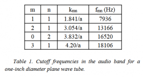
So, if I understand it right, for a 1" PWT there are only four higher order modes that propagate down the tube in the 20 kHz audio band: mn = 11, 21, 02, 31 (and only one of them, 02, being axisymmetric). That means if we don't capture also some of the evanescent modes, all we have for reconstructing the shape of the source wavefront are only those four mode shapes. Hmm, that would be a somewhat crude approximation, wouldn't it.
Last edited:
I tried to calculate the actual decay rate for the first evanescent axi-mode (m=0, n=3) and if I have it correct it would be -45 dBSPL each 10 mm at 10 kHz (-36 dB/10 mm at 20 kHz). Could that be? That's undetectable even at the closest mic position, I'm afraid...
Last edited:
Actually there are three modes (0,0), (0,1), and (0,2). These should certainly be enough to get a description of the shape that is relevant below 20 kHz. The evanescent modes do decay very fast at HFs, but yet in many applications these evanescent modes have been used to give useful information, but perhaps not in this case.
Last edited:
The cut-off of (0,2) (i.e. for kr*a = 7; they start counting n from 1 in the above article) is around 30 kHz, so there is only the planar mode and one non-planar that propagate reasonably far enough (the higher the frequency, the slower the decay). I will definitely try it but based on these number I'm starting to be a bit sceptical.
For the second tube I'm inclined to try more mics placed closer to the source. That will be 1.4" which could be a little easier.
- I should have calculated this before but I really hadn't understood the propagation constants until yesterday 🙂
For the second tube I'm inclined to try more mics placed closer to the source. That will be 1.4" which could be a little easier.
- I should have calculated this before but I really hadn't understood the propagation constants until yesterday 🙂
Last edited:

"... evanescent (0,1)-to-(0,0) conversion"
That is fascinating. Which leads to a question whether an evanescent wave emanating from a driver can excite a propagating mode in a waveguide
That is fascinating. Which leads to a question whether an evanescent wave emanating from a driver can excite a propagating mode in a waveguide
Last edited:
In the simulations I'd like to incorporate a very basic model of a compression driver driven by voltage instead of the constant acceleration boundary elements used so far. Would be someone willing to help me to assemble a lumped element model for this purpose? Basically all I'm interested in is the diaphragm excursion. We know that horns make the drivers more efficient but how much is the excursion actually decreased in practice? For this I would very much appreciate some kick-off - I've never worked with these things (the lumped element models) and don't know where to start...
Here's the ABEC project I've been using to simulate a 1" soft dome tweeter in an axisymmetric waveguide. It incorporates driver and waveguide geometry and an LE-Script for the electrical properties of the tweeter itself.
It's not terribly difficult to setup the LE-Script if you have all the TS parameters, and if can be expanded from what I have here to something much more comprehensive. It's straightforward to add enclosures, filters, and passive components to the LE 'System' model and observe the impact on the simulation.
VACS also has a curve-fitting tool to approximate TS parameters from FR and Impedance graphs, which I've used here.
Attachments
; they start counting n from 1 in the above article)
Which I have concern with since n=0 is a propagating plane wave mode and must be considered because, in our case, it is the dominate mode.
That is fascinating. Which leads to a question whether an evanescent wave emanating from a driver can excite a propagating mode in a waveguide
No. it can't. Not until the frequency is high enough for wave propagation.
In the simulations I'd like to incorporate a very basic model of a compression driver driven by voltage instead of the constant acceleration boundary elements used so far. Would be someone willing to help me to assemble a lumped element model for this purpose? Basically all I'm interested in is the diaphragm excursion.
This is precisely the work that I am doing right now for a client. I have an accurate model in MathCad if you can use that, or I can show you with equations how it's done. Your choice.
Did you see the picture? Evanescent mode converted into (0,0):No. it can't. Not until the frequency is high enough for wave propagation.

- As for the mode indices, I think there's a typo in that article. Anyway, only two axisymmetric modes propagate: (0,0) and (0,1). The mode (0,2) decays already very fast.
Attachments
Last edited:
That would be awesome!... or I can show you with equations how it's done.
Thank you so much! I will go through it.Here's the ABEC project I've been using to simulate a 1" soft dome tweeter in an axisymmetric waveguide. It incorporates driver and waveguide geometry and an LE-Script for the electrical properties of the tweeter itself.
It's not terribly difficult to setup the LE-Script if you have all the TS parameters, and if can be expanded from what I have here to something much more comprehensive. It's straightforward to add enclosures, filters, and passive components to the LE 'System' model and observe the impact on the simulation.
VACS also has a curve-fitting tool to approximate TS parameters from FR and Impedance graphs, which I've used here.
- I'm sure ABEC/AKABAK has all the means how to define the elements directly and elegantly, I just don't know how - I wonder how to enter the compression ratio into the model most easily. I don't need all the phase plug details...
Did you see the picture? Evanescent mode converted into (0,0):
- As for the mode indices, I think there's a typo in that article. Anyway, only two axisymmetric modes propagate: (0,0) and (0,1). The mode (0,2) decays already very fast.
I'd have to look more closely at the derivation of this. I am sure that some small amount of the evanescent wave can be converted into a (0,0) mode if the evanescent wave is not planar - just as shown in the pic. But in all cases it will be very small.
The J0 Bessel Function has a zero slope at k = 0 so this is also a solution, but he seems to have not listed it looking only at the HOMs.
That would be awesome!
See if this helps:
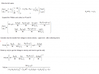
The attached will yield the displacement in a vacuum. If you want a loaded diaphragm then you need to add in the matrices on the right that represent the acoustics. It's not too hard to assume that the load Za is simply Rho-C which is pretty accurate. The real displacement will be 10-20% lower than the vacuum values.
Zm is the total mechanical Z as shown as the upper right element of the diaphragm matrix. "i" is just an index that equates to frequency.
PS. This portion of the model does not contain the compression ratio. That appears as a transformer from the acoustical device to the mechanical diaphragm and increases the Z of the acoustic waveguide device as seen by the diaphragm. I can show you how to do that if you need it.
Attachments
Last edited:
Thanks, I'll have to go through this very slowly... 😱 Right now I don't have a clue what does that all mean. I admire this.
- In the end I'd like to be able to compare different waveguides and their effects on the excursion (for a given driver and SPL) - you know, the "loading" thing. I have the throat radiation impedance calculated that needs to be coupled to the lumped element model of the driver somehow.
- In the end I'd like to be able to compare different waveguides and their effects on the excursion (for a given driver and SPL) - you know, the "loading" thing. I have the throat radiation impedance calculated that needs to be coupled to the lumped element model of the driver somehow.
Last edited:
Again, that is exactly the problem that I am doing, although in mine the waveguide is just a simple one so I don't need a comprehensive model of it. At least not right now, but maybe in the future.
The basic premise of those equations is that every domain, electric (on left), mechanical (middle) and then acoustical (not shown) all have two conjugate variables that are linked via transform matrices. So we have Voltage (E), current (I) in the electric domain, then a Bl transform to the mechanical where we have force (F) and Velocity (v). If the acoustical domain were present then it would be Pressure (P) and Volume Velocity (U) and the coupling would be a matrix of area ratios. My book shows all this in detail.
The basic premise of those equations is that every domain, electric (on left), mechanical (middle) and then acoustical (not shown) all have two conjugate variables that are linked via transform matrices. So we have Voltage (E), current (I) in the electric domain, then a Bl transform to the mechanical where we have force (F) and Velocity (v). If the acoustical domain were present then it would be Pressure (P) and Volume Velocity (U) and the coupling would be a matrix of area ratios. My book shows all this in detail.
Thank you very much so far. I return back to your book regularly. I wish I had a proper education in the field, it would go much smoother for me - who could anticipate I will get this far with this hobby...
Last edited:
- Home
- Loudspeakers
- Multi-Way
- Acoustic Horn Design – The Easy Way (Ath4)