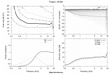
There must be some slight change to the script or setting in the officially released CE360 and the one that was used to produce the graph. The Rad Imp and the directivity above 15K are different and it is not due to the Ath versions as far as I can see as I get the same result on 4.7.0 as you do on 4.8.0.I wonder whether Marcel further changed the configuration vis-a-vis the published one, or whether there is regression in the code between Ath-4.7.1 referenced by Marcel's script and Ath-4.8.0. Regardless, I am rather satisfied with my progress.
Comparison gif attached
Attachments
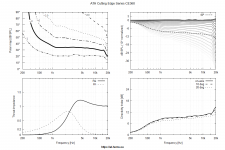
On my website the plots are for a flat source but that also means that the throat angle was set to zero (as is stated there). The published script has a non-zero throat angle, hence the difference. This is something to be adjusted for a driver used, that's not a fixed property of the waveguide. So all the simulations are "correct".
The ABEC.Polars::Offset item is an important one for an infinite baffle case, to not to get behind the baffle plane. In a free-standing case this has much less importance and I doubt it was the real cause. But I don't have an idea what that could be either.
The ABEC.Polars::Offset item is an important one for an infinite baffle case, to not to get behind the baffle plane. In a free-standing case this has much less importance and I doubt it was the real cause. But I don't have an idea what that could be either.
Last edited:
I would not have guessed this to be the reason as in many previous simulations I did not notice a big difference but it is obvious here.The published script has a non-zero throat angle, hence the difference.
In case it wasn't clear my post was not meant to suggest an error, just a point of difference that was not due to the Ath version used.So all the simulations are "correct".
I was not referring to anyone's post in particular, I just wanted to clarify the matter. The differences are due to different throat angles.
BTW, when simulating for a non-zero throat angle, the source shape probably should be set to spherical (Source.Shape = 1) as the best bet, but I'm still not quite sure. Without a real wavefront model this is just a game anyway.
BTW, when simulating for a non-zero throat angle, the source shape probably should be set to spherical (Source.Shape = 1) as the best bet, but I'm still not quite sure. Without a real wavefront model this is just a game anyway.
Hi fluid,
Hi mbat,
Have a pleasant New Years, evening and do not drink and drive; just drink.
Kindest regards,
M
Thank you very much for running the script on Ath-4.8.0 and thus confirming that there is no code regression. That was my concern.There must be some slight change to the script or setting in the officially released CE360 and the one that was used to produce the graph. The Rad Imp and the directivity above 15K are different and it is not due to the Ath versions as far as I can see as I get the same result on 4.7.0 as you do on 4.8.0.
Hi mbat,
Thank you for the explanation.On my website the plots are for a flat source but that also means that the throat angle was set to zero (as is stated there). The published script has a non-zero throat angle, hence the difference. This is something to be adjusted for a driver used, that's not a fixed property of the waveguide. So all the simulations are "correct".
The Offset directive is rather mysterious. Unless I am making another beginners mistake, if I set any value of NormAngle in the ABEC.Polars:SPL, for a free-standing wave-guide the Offset may be omitted and everything works as expected.The ABEC.Polars::Offset item is an important one for an infinite baffle case, to not to get behind the baffle plane. In a free-standing case this has much less importance and I doubt it was the real cause. But I don't have an idea what that could be either.
Yes, the different Source.Shapes make a difference. However, as noted above, my main goal was to replicate your results so that I have a better understanding of the configuration and assure myself that there is no regression before I start experimenting with modelling the wave-guide that I have.BTW, when simulating for a non-zero throat angle, the source shape probably should be set to spherical (Source.Shape = 1) as the best bet, but I'm still not quite sure. Without a real wavefront model this is just a game anyway.
Have a pleasant New Years, evening and do not drink and drive; just drink.
Kindest regards,
M
Greetings all,
I seem to have another problem. I am trying to model an OS wave-guide without any mouth correction, so my wave-guide definition in the configuration file looks like this:
However, executing the configuration results in report of the mouth size 394.59 x 394.59 mm, which is clearly wrong. Referring to the file coord.text, that is passed to the ABEC reveals the problem - the generated curve is not OS, but starts deviating from the OS formula, cf. the attached Excel spreadsheet (change the extension *.txt to xlsx).
From reading the manual, no other directives outside the Horn Geometry - except the Mouth rollback, which is not defined - should affect the shape; however, I am attaching the entire configuration file, in case I missed something.
Kindest regards,
M
I seem to have another problem. I am trying to model an OS wave-guide without any mouth correction, so my wave-guide definition in the configuration file looks like this:
Code:
; M_80
; Ath version 4.8.0

; -------------------------------------------------------
; Waveguide definition
; -------------------------------------------------------

Throat.Angle = 8.0    ; Half the included angle [deg]
Throat.Diameter = 25.4    ; [mm]
Throat.Profile = 1    ; OS-SE
Coverage.Angle = 39.79    ; Half the included angle [deg]

Length = 169.7        ; [mm]

OS.k = 1.00From reading the manual, no other directives outside the Horn Geometry - except the Mouth rollback, which is not defined - should affect the shape; however, I am attaching the entire configuration file, in case I missed something.
Kindest regards,
M
Attachments
It is not mysterious. The distances for the on and off axis measurement points are made from the diaphragm by default. With an infinite baffle the wider angles will end up behind the infinite baffle, by adding the offset to be the length of the waveguide or more the points will be calculated and measured in front of the infinite baffle.The Offset directive is rather mysterious. Unless I am making another beginners mistake, if I set any value of NormAngle in the ABEC.Polars:SPL, for a free-standing wave-guide the Offset may be omitted and everything works as expected.
In a free standing guide this is much less relevant as you are just measuring from a different point of rotation and there is no baffle to be concerned about. Just something to be aware of. Normalization has no effect on this.
Greetings all,
re post # 9,066, it appears that even if not explicitly called in the configuration, the non-mandatory parameters are set to default values.
Hi fluid,
so why, if one omits both the Normalization and the Offset for free standing wave-guide, the SPL is not depicted?
Kindest regards,
M
re post # 9,066, it appears that even if not explicitly called in the configuration, the non-mandatory parameters are set to default values.
Hi fluid,
so why, if one omits both the Normalization and the Offset for free standing wave-guide, the SPL is not depicted?
Kindest regards,
M
That only seems to be the case for you, I am not sure what is going wrong.so why, if one omits both the Normalization and the Offset for free standing wave-guide, the SPL is not depicted?
This is the line I have in my configuration file to generate polar data, no normalization and no offset, works fine as attached
Code:
ABEC.Polars:SPL = {
  MapAngleRange = 0,180,37
  Distance = 2       ; [m]
}
Attachments
That's correct.re post # 9,066, it appears that even if not explicitly called in the configuration, the non-mandatory parameters are set to default values.
Even the "Distance" parameter can be omitted. Then "far-field" data are calculated (i.e. "very far" from the source, adjusted for 1m distance in absolute SPL).
I seem to have another problem. I am trying to model an OS wave-guide without any mouth correction, ...
For that you have to set Term.s = 0 (and of course Rollback = 0, which is the default so you can omit it).
Example: https://www.desmos.com/calculator/w31tzets3j
Last edited:
Hi fluid,
thank you for your attempts to help. Could you please do me a favor, download the configuration file M_80.cfg from post # 9,066 comment out the Normalization and Offset by semicolons and execute it? I have just tried, and again obtained the SPL spectra as in post # 9053.
Hi Marcel,
thank you for the reply. Yes, I had consulted your other document, OS-SE Waveguide, equation (5) and figured it out. And yes, when I had been looking at the default values, I noted the default of 0 for the Rollback.
In that regards, I was looking at the files that Ath generates, and found file coord.txt, which lists the OS-SE curve in terms of y=f(z). There is also a file nodes.txt, which ties the coordinates to nodes. How does Ath generate the file? I was thinking whether it would be possible to use a generic y=f(x) curve and generate a corresponding node file?
Kindest regards,
M
If you want to simulate an arbitrary axisymmetric geometry without digging deeper into ABEC yourself (which is actually pretty easy in that case), the simplest approach would be to modify the file nodes.txt and overwrite the node coordinates, keeping their number the same.
The file nodes.txt defines the node coordinates and the file solving.txt then connects pairs of nodes into BEM elements. You can easily replace content of these files by anything you create. The structure is really simple to use.
The file coords.txt is only for a profile sketch in a report (i.e. a file read by gnuplot).
Last edited:
Hi Marcel,
thank you for the reply.
Referring to the nodes.txt file, the first subset of the nodes (1 - 60, from my configuration file) describe the OS profile, and then the next subset (61 - 123) - as best understood - describe backward the OS offset by a certain amount. Howsoever, this may not be the correct understanding as (i) there are more nodes herein and (ii) several nodes (119 - 121) are in fact negative. So I think some understanding of the nodes is required. I will try to find it.
My interest is more of a curiosity. I have been trying to understand how does Dr. Geddes obtain such a nice response of his Summa. Thus, I started with modelling the OS profile without the end correction (just to familiarize myself with your program), and the OS profile by itself looks rather bad. So I wondered how I could add a circle tangential to the OS that I understand Dr. Geddes uses/ed for the end correction.
Kindest regards,
M
thank you for the reply.
Ha, ha, simple for smart people like yourself, but not for moron (M) like yours truly.The file nodes.txt defines the node coordinates and the file solving.txt then connects pairs of nodes into BEM elements. You can easily replace content of these files by anything you create. The structure is really simple to use.
Referring to the nodes.txt file, the first subset of the nodes (1 - 60, from my configuration file) describe the OS profile, and then the next subset (61 - 123) - as best understood - describe backward the OS offset by a certain amount. Howsoever, this may not be the correct understanding as (i) there are more nodes herein and (ii) several nodes (119 - 121) are in fact negative. So I think some understanding of the nodes is required. I will try to find it.
My interest is more of a curiosity. I have been trying to understand how does Dr. Geddes obtain such a nice response of his Summa. Thus, I started with modelling the OS profile without the end correction (just to familiarize myself with your program), and the OS profile by itself looks rather bad. So I wondered how I could add a circle tangential to the OS that I understand Dr. Geddes uses/ed for the end correction.
Kindest regards,
M
Hi fluid,
re my post # 9,072, please do not bother. I discovered that I installed and old version of VACS; the current one is working.
Kindest regards,
M
re my post # 9,072, please do not bother. I discovered that I installed and old version of VACS; the current one is working.
Kindest regards,
M
You can display both node and element IDs in ABEC visualization (Views->Structure->Nodes, Element indices) so you can orient yourself (it also helps to switch-off the Symmetries). It really is simple - the nodes are defined as "<node_id> <z_mm> <r_mm>" and the elements as "<element_id> <node_id_1> <node_id_2>":
Nodes "Nodes"
Scale=1mm
1 0.000 12.700
2 0.423 12.728
3 0.916 12.773
...
Elements "SD1"
RefNodes="Nodes"
Subdomain=1
1 1 2
2 2 3
...
Nodes "Nodes"
Scale=1mm
1 0.000 12.700
2 0.423 12.728
3 0.916 12.773
...
Elements "SD1"
RefNodes="Nodes"
Subdomain=1
1 1 2
2 2 3
...
Hi Marcel,
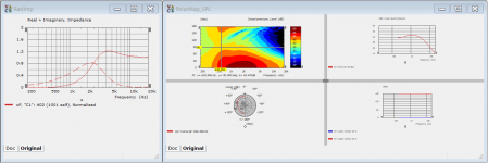
thank you for the visualization. I have a false impression that I start to understand. Looking at the picture:

the nodes P122, P123 are approximating the source, correct? But, what is the purpose of the nodes P120, P121? Could the node 121 be omitted and and node P120 lie on the x-axis directly below the node 119, that is on a line parallel to the y-axis?
Based on your explanation, the elements are now understood.
I know that you are interested in OS/OS-SE, but it seems that with your skills implementing an arbitrary equation should not be difficult.
In any event, I will try to replace the two files; I assume that the rest of the Ath generated files do not need to be modified.
Kindest regards,
M
thank you for the visualization. I have a false impression that I start to understand. Looking at the picture:
the nodes P122, P123 are approximating the source, correct? But, what is the purpose of the nodes P120, P121? Could the node 121 be omitted and and node P120 lie on the x-axis directly below the node 119, that is on a line parallel to the y-axis?
Based on your explanation, the elements are now understood.
I know that you are interested in OS/OS-SE, but it seems that with your skills implementing an arbitrary equation should not be difficult.
In any event, I will try to replace the two files; I assume that the rest of the Ath generated files do not need to be modified.
Kindest regards,
M
P120 and P121 are there to represent the space a compression driver would take, you could, leave them out and go straight back to the zero line.the nodes P122, P123 are approximating the source, correct? But, what is the purpose of the nodes P120, P121? Could the node 121 be omitted and and node P120 lie on the x-axis directly below the node 119, that is on a line parallel to the y-axis?
Hi fluid,
thank you for the explanation.
Now, if that is the case (re nodes P120, P121), could I also omit nodes P119-p117, that is, go directly from the node P116 laying on the y-axes?
Kindest regards,
M
thank you for the explanation.
Now, if that is the case (re nodes P120, P121), could I also omit nodes P119-p117, that is, go directly from the node P116 laying on the y-axes?
Kindest regards,
M
That is not so clear cut, you have to be careful not to have intersecting surfaces that cross over each other as it can cause instability. Test it and see if there is a problem, it will be obvious and generate garbage if there is.Now, if that is the case (re nodes P120, P121), could I also omit nodes P119-p117, that is, go directly from the node P116 laying on the y-axes?
- Home
- Loudspeakers
- Multi-Way
- Acoustic Horn Design – The Easy Way (Ath4)