They do seem to have been RIAA EQ'd before they were cut.
I think you will find all test LP's designed for the general public to be RIAA EQ'd. It's just too technically obscure for someone that wants to evaluate a home system to use anything else. The RCA STR series was designed for professional engineers and includes lots of tracks that are difficult to use/interpret with a non-flat preamp.
"The metal stylus 'carrier' has a lot more surface area and area in contact with the suspension rubber in stylii I have seen tho. They should dominate any head flow."
Bill, I didn't intend to suggest the tie wire itself was the major heatsink, but that it conducts frictional heat away from the magnet (inside the rubber bung) to the metal carrier. In essence, a thermal short around the rubber.
Bill, I didn't intend to suggest the tie wire itself was the major heatsink, but that it conducts frictional heat away from the magnet (inside the rubber bung) to the metal carrier. In essence, a thermal short around the rubber.
I think you will find all test LP's designed for the general public to be RIAA EQ'd.
 I have 4 or 5 vintage test LPs. All are cut with an RIAA curve, as one would expect.
This should have been immediately apparent to those versed in the art from George's pics in #910Ooops! 😱 George's sweeps are indeed RIAA filtered on the LP, if he used a flat preamp. I could only get them flat by running them thru an RIAA curve before analysis. Then they were pretty flat thru most of the range.
Da beachbum pseudo guru was confused and only noted that the FFTs were wonky. 😱
_______________
Seems odd above 18Khz, but that may be an artifact.
Can you give exact details of how you have done this?
Congrats Pano!! You've just re-invented Prof Angelo Farina's method 😱I used HOLMImpulse. It can compare two files to each other, although it isn't always trouble free. I compared George's sweeps to computer generated sine sweeps that I made. But for the graphs posted, George's files were run thru a software RIAA filter to flatten them, which is why they appear flat on the graph.
The funny above 18kHz is because your computer generated sine sweep isn't EXACTLY the same as the original.
Notice how 'all' the 'noise' is gone. The 'swept filter' has a bandwidth of 1/18s = 0.055Hz .. but that means it MUST be accurately placed ... especially at HF.
I didn't think one could get results as good as this as I thought wow & flutter would exceed the 0.055Hz bandwidth but George's system must be extra clean. 🙂
Pano, can you post your computer generated sine sweep and details of EXACTLY how you did it?
It is possible that tweaking this would give us good results up to 20kHz. I was going to count zero crossings in the 18s sweep to do a better one. 😀
It may be that we need to use different methods to get the top 8ve 'right'.
But I now don't have to get off my beach bum **** and dream up 2M FFTs 😎
Pano, could you apply your method to George's measurements from #853 please?
Just a comparison of L & R on
L1st R2nd16.wav
L1st R10th.wav
and then
L1st R34h later.wav
from #864
This won't be good above 15kHz until we tweak your 'computer generated sine sweep' but the differences I expect to see should be at 10kHz too.
If you didn't download the files, I can send them to you if you PM your email
__________________
BTW, as this Angelo's method, those versed in the art can use it to determine THD over 20 - 20k Hz on subsequent playings too. Details in Angelo's paper(s).
I used HOLMImpulse. It can compare two files to each other, although it isn't always trouble free. I compared George's sweeps to computer generated sine sweeps that I made. But for the graphs posted, George's files were run thru a software RIAA filter to flatten them, which is why they appear flat on the graph.
I did look at George's sweeps, they are indeed from 20Hz to 20kHz. They do seem to have been RIAA EQ'd before they were cut.
Pano thanks for the work.
From what I recall from the Digitizing Vinyl thread some months ago, we had come to the conclusion that what Holm does is an RTA and not an FFT.
To summarize:
FFT: bins are of constant width in frequency
RTA: bins are of constant width in octave
White noise: equal energy per Hz bandwidth
Pink noise: equal energy per octave bandwidth
Therefore:
Linear sweeps and white noise:
Appear flat on FFT
Appear rising at 3dB/oct on RTA
Log sweeps and pink noise:
Appear dropping at 3dB/octave on FFT
Appear flat on RTA
The RCA STR series was designed for professional engineers and includes lots of tracks that are difficult to use/interpret with a non-flat preamp.
I need to have the file of a confirmed non-RIAA cut track for to put in order all the assumptions and the wrong practices from my part.
George
Well, Happ 1979 doesn't disclose values needed to settle our disagreement, Richard....... but generally subscribing to it means accepting cantilever flex as a primary mechanism within cartridge mechanics: the principle element of the hf resonant system. Which, apparently, we both do.Actually, my view of the situation has always been Happ which I read when it first came out. IMHO, it is still the most comprehensive and accurate view.
The matter of indentation is worth bottoming out ( 😉 ) because it is practically useful to debunk, or perhaps make sense of, many myths concerning wear, repeat play, rest etc. Also it allows better judgement of the effects of fine radius contact styli.
What I have done is introduce the concept of transverse wave propagation along the cantilever, produced and posted equations describing it, and illustrated it as a short mechanical transmission line that can be reasonably modelled in spice, including boundary conditions of course in the form of source and end termination.In my naive way, I thought your model might be a workable substitute.
What I found, when modelling/sketching a complete AT440 a few years back as a TL model in spice, was only the need for damping as termination - ie no need for reactive termination. Or at least only traces to make the model reasonable. What this suggested, IMO, is that the end terminations probably mostly provide damping, for audioband frequencies and amplitudes. Which, if one reads between the lines of Happ and is more explicit in White, seems consistent to me, and isn't contradicted.
There's no contradiction between the Happ model and the TL model, IMO.
However, it's easy to analyse wave propagation along the cantilever in a TL model, and understand it's artefacts. If one accepts that cantilevers are flexible enough to have an audioband resonant mode, as per Happ, the cantilever is not a rigid body, and stylus motion is not immediately conveyed to the generator end: there's a dispersive phase response, and displacements travel as waves along the cantilever. There are corollaries and consequences to playback performance to deal with. AFAIK these are unaddressed, uncharted waters, and an opportunity for the DSPmeisters to correct, if they are open-minded enough to embrace this and understand what is mechanically going on.
'One can lead a horse to water, but one can't make it drink' 😉
LD
Last edited:
But are you resurrecting your mythical model?.. mostly good stuff ...
What I have done is introduce the concept of transverse wave propagation along the cantilever, produced and posted equations describing it, and illustrated it as a short mechanical transmission line that can be reasonably modelled in spice, including boundary conditions of course in the form of source and end termination.
Pano said:I used HOLMImpulse. It can compare two files to each other, although it isn't always trouble free. I compared George's sweeps to computer generated sine sweeps that I made.
IF HOLMImpulse does the comparison by complex division of the measurement by a reference (Pano's computer generated sweep) it is acting as a Transfer Function Analyzer.Pano thanks for the work.
From what I recall from the Digitizing Vinyl thread some months ago, we had come to the conclusion that what Holm does is an RTA and not an FFT.
These derive an Impulse Response by multiple use of FFTs & other sh*t.
The reference can be any 'wide band' signal .. as long as it is explicitly specified & known. It's not clear from the User Guide what the usual reference signal is but
IF the 'computer generated sweep' is a log sine sweep, it is then doing Angelo's method. This would give the very high immunity from noise that is in Pano's pics.
Angelo's method is the method of choice if Acoustic measurements are required. It is used by beach bums in the wilds of Cooktown as well as the latest Audio Precision. Angelo specifically didn't patent it cos he wanted more people to use it.
This is different from an RTA or FFT analyzer for looking at noise as the 'reference' isn't explicitly known. But a MLS (which has noise type properties) IS explicity known.
ALL 'modern' RTA instruments would use FFTs to create the filters.
Last edited:
Thanks in advance 🙂
George
George,
Here is the promised .wav file, exactly as a Riaa corrected Exponential sweep coming from an LP should be.
When playing this Chirp.wav file, you will have to get the upper FR image of the two below.
The lower FR image is just for completeness and is corrected for the sample frequency which modifies the FR with a sin(x)/x
https://www.dropbox.com/s/55d4picmuhy1frd/chirp.wav?dl=0
Hans

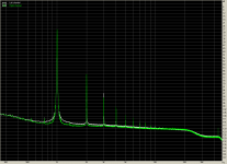
Riaa pre-emphasis was applied through an accurate minimum phase filter, no phase errors within the audio band.The second pic is exactly what I expect for a 18s sweep. It has all the features I describe in #921 & #937.
But how have you applied the RIAA? Was it Minimum Phase?
Size 2^21, no zero padding.How have you done the FFTs? What size? Windowing? Zero padding? bla bla 🙂
Can you be a bit more specific. What noise, where do you see noise ?From this it appears that applying the RIAA pre-emphasis is giving the huge amount of 'noise' .. probably a 'windowing' effect. 😱
Hans
Thank you, Hans. I'm sure that will come in useful one day. I've always wanted to cut a 'proper' test record with 1st hand knowledge of the source.
LD
LD
IF HOLMImpulse does the comparison by complex division of the measurement by a reference (Pano's computer generated sweep) it is acting as a Transfer Function Analyzer.
This is different from an RTA or FFT analyzer for looking at noise as the 'reference' isn't explicitly known. But a MLS (which has noise type properties) IS explicity known.
ALL 'modern' RTA instruments would use FFTs to create the filters.
I only want to avoid or lessen the confusion. 🙂
Please see the similar case with difference in analysis method we had in the past.
Read all the posts btn #262 and #287 (see link below).
Especially the remark of Scott that it is not possible to synchronise anything to a signal with random phase (which applies also to a vinyl recording as phase is much more random than ordered with vinyl playback at the sampling level)
#262
http://www.diyaudio.com/forums/analogue-source/298896-digitizing-vinyl-27.html#post4913272
#287
http://www.diyaudio.com/forums/analogue-source/298896-digitizing-vinyl-29.html#post4917588
George
George,
Here is the promised .wav file,

Thank you Hans.
I'll work on it hopefully in a few hours and report back. (please leave it there till tomorrow)
George
Pano, could you apply your method to George's measurements from #853 please? The differences I expect to see should be at 10kHz too.
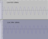
One can do a very simple check and balance that confirms there is no meaningful spectral difference at 10kHZ comparing L1st R10 and 34hr files.
Firstly, visually examine the level of waveforms for the 10kHz sine section in Audacity..... attached is a self-explanatory image that is shows no meaningful difference (!!) Sledgehammer isn't needed for peanuts......
Secondly, run a very short FFT, trading frequency resolution for noise and artefact reduction. Reasonably spanning the 10kHz spot section. Difference I obtain is c 0.04dB@10kHz +/- 0.06dB .........
LD
Attachments
Last edited:
Ditto, the FFTs led me astray. Should have looked at the waveform. Too much time in the Hawaiian sun will fry your brain.Da beachbum pseudo guru was confused and only noted that the FFTs were wonky.
Thanks, that's what I was figuring. I used several different sweeps to compare, all worked, 10 sec, 18 sec, 21sec, but seemed to be off at the top, as you mention.The funny above 18kHz is because your computer generated sine sweep isn't EXACTLY the same as the original.
One thing that shows up everywhere, even FFT, is the big bump at ~32Hz. What is that? You can actually see it modulate the entire sweep waveform.
Files are gone. Maybe I can get them from George and hit them with the sledgehammer.Pano, could you apply your method to George's measurements from #853 please?
Too much time in the Hawaiian sun will fry your brain.
Same with the Athenian sun 😀
One thing that shows up everywhere, even FFT, is the big bump at ~32Hz. What is that? You can actually see it modulate the entire sweep waveform.
It’s one of the artefacts due to the interaction of the vinyl rip file and the stable sinusoidal file you compared it with
(mostly due to phase difference. You can check this out by choosing a slightly different time point to start your reference file. The bump will move in frequency)
Files are gone. Maybe I can get them from George and hit them with the sledgehammer.
Please wait a few hours .
I will post some more robust test files that you can hammer hard.
George
Thanks George.
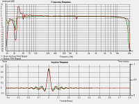
I realized that the FR plots I posted are inverted. That's because I was using the vinyl sweeps as the reference, and comparing a perfect sweep to them. So I had to flip the response. See below, as these seem a lot more believable. Still not sure about what's going on circa 30Hz.
BTW, these are 1/12th octave smoothed.
Attachments
If I will be tempted by the masochistic lust to repeat the test, I will do it with the Shure M97 cartridge reading a 1KHz track from my other test record (UAT).
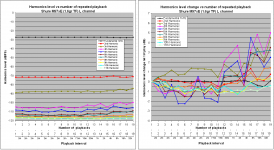
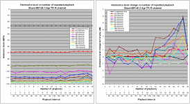
The third and last test run.
Shure M97xE cartridge on Kenwood KD-3100 turntable, to Hagerman Bugle RIAA pre, to M-Audio Audiophile USB card. 24bit/96KHz recordings.
UAT Side 1 Track 1 1KHz @ 7cm/s (2minutes track)
I exercised the cartridge by playing for 15 minutes a music vinyl LP.
Then I played Side 1 Track 1 (1kHz @ 7cm/s ) from “The Ultimate Analog Test LP” for ten consecutive times. Repetition interval 2 minutes.
Then, I played the same track after 15min. and progressively doubling the interval time to 30min, 1hour, 2 hours, 4hours, 8hours, 16hours, 32hours (again exercising the cartridge by playing for 15 minutes the same music vinyl LP).
22.8d Celcius ambient temp for 1 to 15 plays.
22.7d Celcius ambient temp for play 16 (after 4 hours).
22.6d Celcius ambient temp for play 17 (after 8 hours).
23.8d Celcius ambient temp for play 18 (after 16 hours).
25.4d Celcius ambient temp for play 19 (after 32 hours).
Again I used FFT (65536 samples and a lot of zoom-in) to read the peaks from the 1kHz and it’s harmonics on each recording. I entered the data in excel and plotted these diagrams.
1
https://www.dropbox.com/s/w0gi2gz0uzb1amj/1.wav?dl=0
2
https://www.dropbox.com/s/e9itbrtd9a2kh9f/2.wav?dl=0
3
https://www.dropbox.com/s/x4utiubbher1szv/3.wav?dl=0
4
https://www.dropbox.com/s/ksqn2sn3uuvh850/4.wav?dl=0
5
https://www.dropbox.com/s/d16ad4h8nwz3kmy/5.wav?dl=0
6
https://www.dropbox.com/s/gd8nhjz3fs4gn2k/6.wav?dl=0
7
https://www.dropbox.com/s/v149ygqs0x4pybf/7.wav?dl=0
8
https://www.dropbox.com/s/dsxoa6brururs1e/8.wav?dl=0
9
https://www.dropbox.com/s/158ej5exm7pbtx1/9.wav?dl=0
10
https://www.dropbox.com/s/ukavewmugh04cmx/10.wav?dl=0
11 after 7.5 minutes
https://www.dropbox.com/s/uk9lv6k2y74ry5y/11-7_5m.wav?dl=0
12 after 15 minutes
https://www.dropbox.com/s/9b5a6qoz9h4eo6g/12-15m.wav?dl=0
13 after 30 minutes
https://www.dropbox.com/s/jp78rekju5crjah/13-30m.wav?dl=0
14 after 1hour
https://www.dropbox.com/s/k5qrzfjvayf7ffw/14-1h.wav?dl=0
15 after 2 hours
https://www.dropbox.com/s/vg5028t4o5gsmmt/15-2h.wav?dl=0
16 after 4 hours
https://www.dropbox.com/s/mm5m7oyfi2hr1ff/16-4h.wav?dl=0
17 after 8 hours
https://www.dropbox.com/s/xh2uszggztk0zt7/17-8h.wav?dl=0
18 after 16 hours
https://www.dropbox.com/s/maodzug050smh0i/18-16h.wav?dl=0
19 after 32 hours
https://www.dropbox.com/s/vm0uuznj7ur0mta/19-32h.wav?dl=0
George
Attachments
- Home
- Source & Line
- Analogue Source
- mechanical resonance in MMs