Is not certain a place to write certain compliments but only a interchanging opinions in quiet moods
This is not an interchange of opinions. It is a pair of monologues. I don't think you read the posts of others.
And, surprise, technical facts are not 'opinion'- they are not up for negotiation.
As intelligent people we can expect that we are willing to learn from each other. If that is not the case, it gets frustrating.
Jan
Under Shannon-Nyquist's hypothesis, quantization process is lossless and transformation is biunique.
So each signal has one, and only one, equivalent discrete transform. And vice versa.
There's dualism between the two domains.
So each signal has one, and only one, equivalent discrete transform. And vice versa.
There's dualism between the two domains.
going to post 49
Under Shannon-Nyquist's hypothesis, quantization process is lossless and transformation is biunique.
So each signal has one, and only one, equivalent discrete transform. And vice versa.
There's dualism between the two domains.
Shannon
Si ma io sto parlando di altro tipo di problema vai al post 49
e segui gli step
è il motivo per cui si fanno i covertitori nos a parer mio
Tra superarlo e capirlo però ce ne passa. 🙂
Il tuo errore è di base e te lo stanno dicendo in molti.
Per il resto ci sono i libri e una solida dimostrazione matematica che non lascia spazio ad interpretazione.
Inoltre in precedenza ti ho postato un video pratico, se non ti piace la teoria. 😉
Si ma io sto parlando di altro tipo di problema vai al post 49
e segui gli step
è il motivo per cui si fanno i covertitori nos a parer mio
Im sorry to use italian
Excuse me for using Italian......Please reread the rules on use of English.
The plot at post #49 isn't the sampled version of a 15kHz pure sinewave.
The correct plot is from #51 by peufeu.
In fact, sampling produces dots (with lines), not curves.
Example:
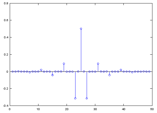
Your plot seems an AM modulation. 🙂
The correct plot is from #51 by peufeu.
In fact, sampling produces dots (with lines), not curves.
Example:
Your plot seems an AM modulation. 🙂
Last edited:
So you're saying that the two signals don't have the same signal power?Triangle wave have 3 orders on Fourier transfer so high
Square wave have 5 orders on Fourier transfer so high
If they have a 10khz of fo on spectrum analysis you find
20Khz 30khz etc...
Over about 20Khz you have Aliasing effect
you have lost othres steps ...
Follow all steps and conclusions
Oh do you knew a discrete sinc ....The plot at post #49 isn't the sampled version of a 15kHz pure sinewave.
The correct plot is from #51 by peufeu.
In fact, sampling produces dots (with lines), not curves.
Example:
Your plot seems an AM modulation. 🙂
Follow all steps and conclusions
Last edited:
Example of code to show a 15kHz sinewave sampled at 44100Hz is:
And the plot is:
Adjust that code for your purpose.
PS: as written, your code plots nothing
Code:
t  = [ 0 : 1 : 40 ];           % Time Samples
f  = 15000;                       % Input Signal Frequency
fs = 44100;                    % Sampling Frequency
x = sin(2*pi*f/fs*t);        % Generate Sine Wave
figure(1);
stem(t,x,'r');                  % View the samples
figure(2);
stem(t*1/fs*1000,x,'r');  % View the samples
hold on;
plot(t*1/fs*1000,x);        % Plot Sine Wave
And the plot is:
An externally hosted image should be here but it was not working when we last tested it.
Adjust that code for your purpose.
PS: as written, your code plots nothing
Last edited:
Without dots you must reduce scale (plot less samples):
And you got something simpler to view but more difficult to understand, because Octave auto-link samples and in reality ADCs don't do that:
In reality sampling is this:
The same code of previous post, without the last line.
I think that the major problem those images is the scale for X in frequency domain 🙂
Code:
fs = 44100; %44100Hz sampling frequency
f = 15000;
t = (0:50-1)/fs;
x = sin(2*pi*f*t);
plot(t,x)
And you got something simpler to view but more difficult to understand, because Octave auto-link samples and in reality ADCs don't do that:
An externally hosted image should be here but it was not working when we last tested it.
In reality sampling is this:
An externally hosted image should be here but it was not working when we last tested it.
The same code of previous post, without the last line.
Code:
t  = [ 0 : 1 : 40 ];           % Time Samples
f  = 15000;                       % Input Signal Frequency
fs = 44100;                    % Sampling Frequency
x = sin(2*pi*f/fs*t);        % Generate Sine Wave
figure(1);
stem(t,x,'r');                  % View the samples
figure(2);
stem(t*1/fs*1000,x,'r');  % View the samples
hold on;
I think that the major problem those images is the scale for X in frequency domain 🙂
Last edited:
Now do the same thing, but with two sine waves at 15kHz and 29.1kHz. Get the amplitudes right, and you should see a similar plot. This is because (ignoring higher images) 15kHz and 29.1kHz sampled at 44.1kHz are indistinguishable from 15kHz sampled at 44.1kHz.
Example of code to show a 15kHz sinewave sampled at 44100Hz is:
And the plot is:Code:t = [ 0 : 1 : 40 ]; % Time Samples f = 15000; % Input Signal Frequency fs = 44100; % Sampling Frequency x = sin(2*pi*f/fs*t); % Generate Sine Wave figure(1); stem(t,x,'r'); % View the samples figure(2); stem(t*1/fs*1000,x,'r'); % View the samples hold on; plot(t*1/fs*1000,x); % Plot Sine Wave
An externally hosted image should be here but it was not working when we last tested it.
Adjust that code for your purpose.
icrease t from 40 to 400
PS: as written, your code plots nothing
Code:
t  = [ 0 : 1 : 200 ];           % Time Samples
f  = 15000;                       % Input Signal Frequency
fs = 44100;                    % Sampling Frequency
x = sin(2*pi*f/fs*t);        % Generate Sine Wave
figure(1);
stem(t,x,'r');                  % View the samples
figure(2);
stem(t*1/fs*1000,x,'r');  % View the samples
hold on;
An externally hosted image should be here but it was not working when we last tested it.
So, where's the problem?
Are you afraid of points involution?
It's an optical illusion 😉
Real FFT of this signal is a line centered in +-n*fc (quantization become spectrum replication) with n from 1 to infinite.
To see all aliases, you must use a proper command to obtain proper X-axis values (negative too).
AHAHAHA you are fine person
Optical illusion ?!? hey guy what is described trough the samples, the modulation results are two sine in opposition of phase on fft you cant see them -fd cancel +fd
but these only on ideal system adc or dac
Code:t = [ 0 : 1 : 200 ]; % Time Samples f = 15000; % Input Signal Frequency fs = 44100; % Sampling Frequency x = sin(2*pi*f/fs*t); % Generate Sine Wave figure(1); stem(t,x,'r'); % View the samples figure(2); stem(t*1/fs*1000,x,'r'); % View the samples hold on;An externally hosted image should be here but it was not working when we last tested it.
So, where's the problem?
Are you afraid of points involution?
It's an optical illusion 😉
Real FFT of this signal is a line centered in +-n*fc (quantization become spectrum replication) with n from 1 to infinite.
To see all aliases, you must use a proper command to obtain proper X-axis values (negative too).
Optical illusion ?!? hey guy what is described trough the samples, the modulation results are two sine in opposition of phase on fft you cant see them -fd cancel +fd
but these only on ideal system adc or dac
Optical illusion ?!? hey guy what is described trough the samples, the modulation results are two sine in opposition of phase on fft you cant see them -fd cancel +fd
There is no modulation, which is why you can't see them on FFT. It is an optical illusion, like this :

Street furniture knows Shannon's theorem :

I think in the end we need the vinyl for Hi-end audio chains
This is the problem. You don't.
Digital works. You don't like that. You try and find some technical objection, but you found nothing, because digital works, which you forgot when you 'discovered' this BS.
There is no modulation, which is why you can't see them on FFT. It is an optical illusion, like this :
I admire your tenacity in the face of an abyss.
I admire your tenacity in the face of an abyss.
Yeah, I'm outta here 😀
- Status
- Not open for further replies.
- Home
- Member Areas
- The Lounge
- Shannon ad fc/2 tricks