No. Collaboration involves communication, and learning from each other. You have repeatedly refused to engage in meaningful communication. You just keep asserting your own wrong view. We keep telling you to do some more reading so your understanding grows. You seem unwilling or unable to do this.gumo73 said:I'm collaborative man because others have the experince to do the right measurements
to post the impact of this .
There is nothing "inexplicable" about sampling theory, but there are aspects of it which some people find to be surprising or even counter-intuitive. The solution is to have a better informed intuition, by properly understanding the maths. As I keep saying, you need to learn about images. Some people may find it easier to start by properly understanding aliasing, provided they don't then get images and aliases mixed up in their mind.
A little more step
This is the FFT results for fo=15khz nearest fc/3.
This below is a working progress matlab/octave script rename it filename.m
fft_xt is the fft of sine acquisition .
fft_xt1 is the fft of first modulation
fft_xt1+xt2 is the print of fft of first modulation and second modulation on the same graph
fft_xt1+xt2+xt3 is the print of first second and third modulation on the same graph
For DF96
If you think about being able to explain me these results
Noise doesn't come from the moon...
If you know signals theory
Attachments

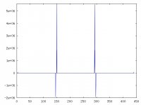
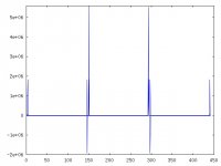
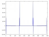
Your first plot shows the original 15kHz signal, plus the first image at 29.1kHz. Exactly as expected. The second plot shows two signals, and two images, exactly as expected. etc.
Now apply a reconstruction filter, which will remove everything above 22.05kHz. You get the original signals. Why do you find this so difficult to grasp?
Now apply a reconstruction filter, which will remove everything above 22.05kHz. You get the original signals. Why do you find this so difficult to grasp?
Ok
But if the dac is not ideal ? was heppen ?
Your first plot shows the original 15kHz signal, plus the first image at 29.1kHz. Exactly as expected. The second plot shows two signals, and two images, exactly as expected. etc.
Now apply a reconstruction filter, which will remove everything above 22.05kHz. You get the original signals. Why do you find this so difficult to grasp?
But if the dac is not ideal ? was heppen ?
A non-ideal DAC produces distortion, just like every other nonlinear component. So what? DACs are much closer to being linear than, say, an MM playing an LP on a turntable.
I need your help
Do oyu can help me to do a reconstruction filter not ideal ?
Do you have a matlab iteration for some 4x not ideal ?
In this post you apply sinc ( ideal case)
Thanks to advance
Here ya go.
First I create an "analog" signal (it's just oversampled but that's well enough so it looks pleasing to the eye).
Since it is a pure 15k sine, it is perfectly bandlimited and by sampling it at 44.1k, no information is lost. The samples are the black dots.
It looks like there is a beat frequency, visually.
Note I do not display lines between samples because it makes no sense. Lines should only be displayed when the oversampling is high enough (or the signal slow enough) that linear interpolation doesn't give too much bogus results. Which is obviously not the case here.
The sinc reconstruction brings back the original "analog" signal, as you see. No problem.
Code:from numpy import * import matplotlib.pyplot as plt # create "analog" signal def make_signal( Fs, NSamples, freq, oversampling ): Fs *= oversampling NSamples *= oversampling t = arange(NSamples) * (1.0/Fs) return t, cos( 2*pi*freq*t ) Fs = 44100. NSamples = 100 freq = 15000. plt.figure(1) plt.subplot(3,1,1) analog_t, analog_signal = make_signal( Fs, NSamples, freq, 16 ) plt.plot( analog_t, analog_signal, "b-", label='"analog" signal' ) digital_t, digital_signal = make_signal( Fs, NSamples, freq, 1 ) plt.plot( digital_t, digital_signal, "ko", label='"digital" signal' ) plt.xlabel("time (s)") plt.title("signal and samples") plt.legend() plt.tight_layout() plt.subplot(3,1,2) reconstruct_oversample_ratio = 8 reconstruct_length = 32 * reconstruct_oversample_ratio impulse = sinc( (1.0/reconstruct_oversample_ratio) * arange( -reconstruct_length, reconstruct_length ) ) plt.plot( impulse ) plt.xlabel("sample #") plt.title("reconstruction filter") plt.tight_layout() plt.subplot(3,1,3) # recondtruct sampled signal # first insert zeros digital_signal_padded = zeros( NSamples * reconstruct_oversample_ratio ) digital_signal_padded[::reconstruct_oversample_ratio] = digital_signal # then convolve (very dumb method) reconstructed = convolve( digital_signal_padded, impulse ) plt.plot( reconstructed ) plt.title( "reconstructed" ) plt.show()
Do oyu can help me to do a reconstruction filter not ideal ?
Do you have a matlab iteration for some 4x not ideal ?
In this post you apply sinc ( ideal case)
Thanks to advance

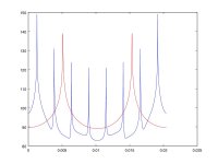
Nearest fc/4
This is a linear digital interpolation at 11Khz
Is a working progress.
I have some problems with right scaling of fft graphs , need help on
this print...
Below image of fft-signals original and oversampled at 4X
txt as filename.m of octave
This is a linear digital interpolation at 11Khz
Is a working progress.
I have some problems with right scaling of fft graphs , need help on
this print...
Below image of fft-signals original and oversampled at 4X
txt as filename.m of octave
Attachments
I think if is possible to emulate a real dac is possible
to evalutate was heppen at values nearest fc/4 in
I this place are present 4 modulation and produce noise
bleow
That noise is due to high jitter.
noise
I'm find the source a simple time shift can create many beats.
Help me with last octave/matlab script !!
That noise is due to high jitter.
I'm find the source a simple time shift can create many beats.
Help me with last octave/matlab script !!
noise
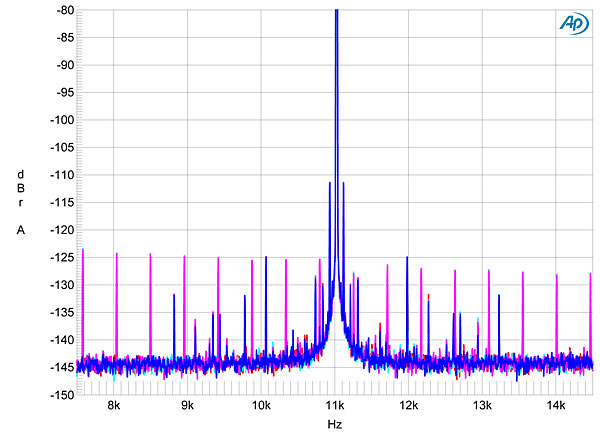
S/N on nos and oversampling is the same about 45dB
But on fft of oversampling there are many sine wave than on nos fft about jitter .
For best interpolation i think the sinc is only one by one for all samples .
Below first is of the nos DAC and second of oversampling DAC.
S/N on nos and oversampling is the same about 45dB
But on fft of oversampling there are many sine wave than on nos fft about jitter .
For best interpolation i think the sinc is only one by one for all samples .
Below first is of the nos DAC and second of oversampling DAC.
Attachments

Last edited:
Last Octave script
In the end i think the multiphase system transport the information about maximum value.
The jitter have a modulation effect on the center of
the multi phase system and need a very highest precision
to have a very low modulation frequencies .😀
Rename the script from name.txt to name.m
and see the results
Attachments
Visual effects and real effects
By this simple example is possible to see the multi phase sine
systems inside the signal of a sampled sine inside shannon band
fc/2 .
This is one of many others sine
Results and the Spreadsheet 🙂
Sorry for my bad English😀
By this simple example is possible to see the multi phase sine
systems inside the signal of a sampled sine inside shannon band
fc/2 .
This is one of many others sine
Results and the Spreadsheet 🙂
Sorry for my bad English😀
Attachments

Calculus
For obtain the image you need to generate a sampled
sine by this calculus
fo=12500hz v(kt)=sin(2*3.14*fo*kTc)
k=1,2,3,........,n
Where Tc is a 1/Fc and Fc=44100hz (sample rate freq.)
Set up a level variable between (0;1) for example vf
and create the output values v(kt) filtrated by level
v(kt) if v(kt)>vf or 0 in other case
Print result by Spreadsheet graph, and see results....🙂
I think on NOS dac the noise around 50-100hz is coming out
from this point.🙂
By this simple example is possible to see the multi phase sine
systems inside the signal of a sampled sine inside shannon band
fc/2 .
This is one of many others sine
Results and the Spreadsheet 🙂
Sorry for my bad English😀
For obtain the image you need to generate a sampled
sine by this calculus
fo=12500hz v(kt)=sin(2*3.14*fo*kTc)
k=1,2,3,........,n
Where Tc is a 1/Fc and Fc=44100hz (sample rate freq.)
Set up a level variable between (0;1) for example vf
and create the output values v(kt) filtrated by level
v(kt) if v(kt)>vf or 0 in other case
Print result by Spreadsheet graph, and see results....🙂
I think on NOS dac the noise around 50-100hz is coming out
from this point.🙂
- Status
- Not open for further replies.
- Home
- Member Areas
- The Lounge
- Shannon ad fc/2 tricks