The recent disputes regarding the lowest-noise operational amplifier, mainly as a single-stage phono EQ, have prompted me to ask:
how can I get a concrete reference point as quickly as possible, comparing individual types of OP?
Whether absolute values are generated is irrelevant, it is the comparison that is of interest. The type with the highest SNR wins.
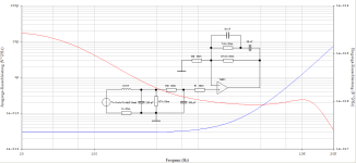
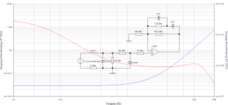
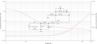
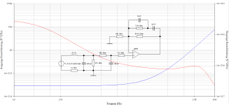
SCHEMATIC

The win32 program noise.exe opens a cmd and presents itself as follows:
OPu=
OPi=
G1k=
Rq=
Ltc=
Rdc=
R1=
R2=
R3=
df=
T=
1.730631e-007[V] 1.747937e-005[V] 88.53378[dB]
99.0099 7500 3112.292 10000 100 3333 47000
OPu=
C:\Windows\System32>
enter as a normal floating point variable or confirm with the enter key, the rest will become clear as you play.
#
Have fun with it - and of course I cannot guarantee correctness and correct operation.
However,
the theoretical calculation of the noise, manifested here in the SNR (last output value of the first line), is actually trivial.
Nevertheless,
I could have made a dozen mistakes.
HBt.
how can I get a concrete reference point as quickly as possible, comparing individual types of OP?
Whether absolute values are generated is irrelevant, it is the comparison that is of interest. The type with the highest SNR wins.
SCHEMATIC
The win32 program noise.exe opens a cmd and presents itself as follows:
OPu=
OPi=
G1k=
Rq=
Ltc=
Rdc=
R1=
R2=
R3=
df=
T=
1.730631e-007[V] 1.747937e-005[V] 88.53378[dB]
99.0099 7500 3112.292 10000 100 3333 47000
OPu=
C:\Windows\System32>
enter as a normal floating point variable or confirm with the enter key, the rest will become clear as you play.
- OPu stands for en in V/sqrt(Hz) and OPi stands for In in A/sqrt(Hz) of the operational amplifier used
- Rq stands for the resulting effective resistance of our pickup, alternatively a DC resistance (in ohms) and a coil inductance (in H) can be specified
- df stands for the desired bandwidth of our thermal noise (in Hz)
- T for the temperature (in °C) ...
#
Have fun with it - and of course I cannot guarantee correctness and correct operation.
However,
the theoretical calculation of the noise, manifested here in the SNR (last output value of the first line), is actually trivial.
Nevertheless,
I could have made a dozen mistakes.
HBt.
Attachments

Thermal noise only, band-limited to 2kHz:
1)
OPA627 0dB
OPu=8e-9
OPi=1.6e-15
8.007577e-009[V] 8.087653e-007[V] 115.2279[dB]
99.0099 5000000 3112.292 10000 100 3333 47000
2)
TL071 -4.4dB
OPu=18e-9
OPi=10e-15
1.333835e-008[V] 1.347174e-006[V] 110.7958[dB]
99.0099 1800000 3112.292 10000 100 3333 47000
3)
AD825 -6.2dB
OPu=12e-9
OPi=10e-15
1.632881e-008[V] 1.64921e-006[V] 109.0388[dB]
99.0099 1200000 3112.292 10000 100 3333 47000
4)
LM741 -18.5dB
OPu=20e-9
OPi=0.3e-12
6.775719e-008[V] 6.843477e-006[V] 96.67876[dB]
99.0099 66666.67 3112.292 10000 100 3333 47000
5)
OP27 -26.7dB
OPu=3e-9
OPi=0.4e-12
1.730631e-007[V] 1.747937e-005[V] 88.53378[dB]
99.0099 7500 3112.292 10000 100 3333 47000
6)
NE5534 -26.8dB
OPu=5e-9
OPi=0.7e-12
1.760225e-007[V] 1.777827e-005[V] 88.38651[dB]
99.0099 7142.857 3112.292 10000 100 3333 47000
7)
LT1028 -31dB
OPu=0.85e-9
OPi=1e-12
2.81056e-007[V] 2.838666e-005[V] 84.32201[dB]
99.0099 850 3112.292 10000 100 3333 47000
The ranking, with the OPA627 as a reference (in PMA's OpenAmpOne dimensioning), the LT1028 brings up the rear in terms of noise, even a 741 performs much better here with an MM -> the OPs are assumed to be ideal.
Whether the simplest and most approximate calculation with the noise source models provides us with a correct indication is still up in the air.
HBt.
Let's compare theoretically (and scaled) the real SNR (unweighted) between a 47k and a 150k termination.
OPu=8e-9
OPi=1.6e-15
G1k=100
Rq=
Ltc=0.6
Rdc=600
R1=47000
R2=100
R3=
df=20000
T=27
2.872449e-008[V] 2.901174e-006[V] 104.0496[dB]
99.0099 5000000 3530.61 10000 100 3817.368 47000
OPu=8e-9
OPi=1.6e-15
G1k=100
Rq=
Ltc=0.6
Rdc=600
R1=150000
R2=100
R3=
df=20000
T=27
3.028616e-008[V] 3.058902e-006[V] 104.0498[dB]
99.0099 5000000 3722.63 10000 100 3817.368 150000
OP is OPA627 ...
and there is no real difference with a Difet.
OPu=8e-9
OPi=1.6e-15
G1k=100
Rq=
Ltc=0.6
Rdc=600
R1=47000
R2=100
R3=
df=20000
T=27
2.872449e-008[V] 2.901174e-006[V] 104.0496[dB]
99.0099 5000000 3530.61 10000 100 3817.368 47000
OPu=8e-9
OPi=1.6e-15
G1k=100
Rq=
Ltc=0.6
Rdc=600
R1=150000
R2=100
R3=
df=20000
T=27
3.028616e-008[V] 3.058902e-006[V] 104.0498[dB]
99.0099 5000000 3722.63 10000 100 3817.368 150000
OP is OPA627 ...
and there is no real difference with a Difet.
Let's compare theoretically (and scaled) the real SNR (unweighted) between a 47k and a 150k termination.
OPu=0.85e-9
OPi=1e-12
G1k=100
Rq=
Ltc=0.6
Rdc=600
R1=47000
R2=10
R3=
df=20000
T=27
9.697e-007[V] 9.793969e-005[V] 73.48194[dB]
9.90099 850 3530.61 1000 10 3817.368 47000
OPu=0.85e-9
OPi=1e-12
G1k=100
Rq=
Ltc=0.6
Rdc=600
R1=150000
R2=10
R3=
df=20000
T=27
1.000789e-006[V] 0.0001010797[V] 73.66784[dB]
9.90099 850 3722.63 1000 10 3817.368 150000
OP is LT1028 ...
and there is also no real difference with "a noisy" bjt.
The essential point is equal (noise) source impedances at the inputs of the operational amplifier, df=2kHz
LT1028
OPu=0.85e-9
OPi=1e-12
G1k=100
Rq=10
Ltc=
Rdc=
R1=47000
R2=10
R3=
df=
T=
1.950825e-009[V] 1.970334e-007[V] 128.0868[dB]
9.90099 850 9.997872 1000 10 10 47000
OPA627
OPu=8 e-9
OPi=1.6e-15
G1k=100
Rq=10
Ltc=
Rdc=
R1=47000
R2=10
R3=
df=
T=
2.57316e-011[V] 2.598892e-009[V] 165.6818[dB]
9.90099 5000000 9.997872 1000 10 10 47000
Here, too, the Difet from formerly BurrBrown is way ahead. However, all of the listed OPs are suitable for building an RIAA EQ, whether it is also possible with a single LM741 is up to your imagination.
HBt.
OPu=0.85e-9
OPi=1e-12
G1k=100
Rq=
Ltc=0.6
Rdc=600
R1=47000
R2=10
R3=
df=20000
T=27
9.697e-007[V] 9.793969e-005[V] 73.48194[dB]
9.90099 850 3530.61 1000 10 3817.368 47000
OPu=0.85e-9
OPi=1e-12
G1k=100
Rq=
Ltc=0.6
Rdc=600
R1=150000
R2=10
R3=
df=20000
T=27
1.000789e-006[V] 0.0001010797[V] 73.66784[dB]
9.90099 850 3722.63 1000 10 3817.368 150000
OP is LT1028 ...
and there is also no real difference with "a noisy" bjt.
The essential point is equal (noise) source impedances at the inputs of the operational amplifier, df=2kHz
LT1028
OPu=0.85e-9
OPi=1e-12
G1k=100
Rq=10
Ltc=
Rdc=
R1=47000
R2=10
R3=
df=
T=
1.950825e-009[V] 1.970334e-007[V] 128.0868[dB]
9.90099 850 9.997872 1000 10 10 47000
OPA627
OPu=8 e-9
OPi=1.6e-15
G1k=100
Rq=10
Ltc=
Rdc=
R1=47000
R2=10
R3=
df=
T=
2.57316e-011[V] 2.598892e-009[V] 165.6818[dB]
9.90099 5000000 9.997872 1000 10 10 47000
Here, too, the Difet from formerly BurrBrown is way ahead. However, all of the listed OPs are suitable for building an RIAA EQ, whether it is also possible with a single LM741 is up to your imagination.
HBt.
Update V1.1
In the first approach, three substitute sources are formed; they do not correlate. In the second approach, all sources are consistently shifted first and the density is used in the calculation; now everything correlates. The results of the alternative method (superposition and correlating) can now be found in the third row.
HBt.
#
OPA627 in PMA's OpenAmpOne
OPu=8e-9
OPi=1.6e-15
G1k=
Rq=
Ltc=
Rdc=
R1=
R2=
R3=
df=20000
T=
2.532218e-008[V] 2.55754e-006[V] 105.2279[dB]
99.0099 5000000 3112.292 10000 100 3333 47000
1.639439e-006[V] 0.0001655833[V] 69.00397[dB]
OPu=8e-9
OPi=1.6e-15
G1k=
Rq=
Ltc=
Rdc=
R1=
R2=
R3=
df=2000
T=
8.007577e-009[V] 8.087653e-007[V] 115.2279[dB]
99.0099 5000000 3112.292 10000 100 3333 47000
5.184361e-007[V] 5.236204e-005[V] 79.00397[dB]
... with good correspondence to the measured SNR.
@MarcelvdG
How would you calculate?
Attachments
Last edited:
This is the result for the old OP27 (df=2kHz):
1.730631e-007[V] 1.747937e-005[V] 88.53378[dB]
99.0099 7500 3112.292 10000 100 3333 47000
3.826304e-007[V] 3.864567e-005[V] 81.64228[dB]
This result was confirmed by Pavel M. a few days ago. This is very interesting because this is the original application note, which can be found in the OP27 data sheet.
OAone uses an additional buffer in the feedback path and inevitably also a DC servo.
kindly,
HBt.
The recent disputes regarding the lowest-noise operational amplifier, mainly as a single-stage phono EQ, have prompted me to ask:
how can I get a concrete reference point as quickly as possible, comparing individual types of OP?
Whether absolute values are generated is irrelevant, it is the comparison that is of interest. The type with the highest SNR wins.
But you haven't provided the source code so we have no idea if you've done the right calculation! Why not use something portable too, like Python or even a spreadsheet, then it would run on other OS's.Have fun with it - and of course I cannot guarantee correctness and correct operation.
However,
the theoretical calculation of the noise, manifested here in the SNR (last output value of the first line), is actually trivial.
Nevertheless,
I could have made a dozen mistakes.
HBt.
2kHz? Why? And its not thermal noise only is it as the device current and voltage noise must be in there or what's the point?Thermal noise only, band-limited to 2kHz:
Also if you are modelling the inductance of the cartridge you are interested in the frequency distribution of the noise, if so then surely it makes sense to model the RIAA network which also contributes to the noise frequency distribution?
Had a play at a Python noise plotting function, source provided...
Setup a few noise models for opamps, graph results:

The variation in voltage noise is fairly small except for the glaring exception of the uA741 (!), but the current noise contributions are very different - just look at the massive improvement of switching to NE5534A from LM4562, two bipolar opamps, and the fact the FET opamps are free from the HF bump.
I plotted both input and output referred noise densities, with an assumption of 60-fold gain at 1kHz (35.56dB).
In practice the higher frequency noise is the most audible (ears more sensitive, less competition from other sources), so the lesson is current noise is everything in a MM preamp, so long as you don't use a uA741...
Also I don't know of any bipolar opamp that beats the NE5534A for this application.
Setup a few noise models for opamps, graph results:
The variation in voltage noise is fairly small except for the glaring exception of the uA741 (!), but the current noise contributions are very different - just look at the massive improvement of switching to NE5534A from LM4562, two bipolar opamps, and the fact the FET opamps are free from the HF bump.
I plotted both input and output referred noise densities, with an assumption of 60-fold gain at 1kHz (35.56dB).
In practice the higher frequency noise is the most audible (ears more sensitive, less competition from other sources), so the lesson is current noise is everything in a MM preamp, so long as you don't use a uA741...
Also I don't know of any bipolar opamp that beats the NE5534A for this application.
Code:
from math import pi, sqrt, log10
import numpy as np
import matplotlib.pyplot as plt


# setup cartridge parameters
Ls = 0.5
Rs = 1000.0

# load resistor
Rl = 47e3  # load resistance (constant)


# RIAA response function

POLE1 = 1 / 3180e-6
ZERO  = 1 / 318e-6
POLE2 = 1 / 75e-6

def raw_RIAA_gain (f):
    w = 2 * pi * f
    s = 1j * w
    numerator = (s - ZERO)
    denominator = (s - POLE1) * (s - POLE2)
    return abs (numerator / denominator)

GAIN_1K = raw_RIAA_gain (1e3)

# normalize to a gain of 60 at 1k, i.e. 35.56dB
def RIAA_gain (f):
    return 60 * raw_RIAA_gain (f) / GAIN_1K


# auxiliary functions
def sqr (a):
    return a * a

def Rnoise (R):
    T = 298.0
    k = 1.3806e-23
    Vn = sqrt (4 * k * T * R)
    return Vn

def Parallel (Z1, Z2):
    return Z1 * Z2 / (Z1 + Z2)


def input_noise_density (Ls, Rs, Ve, Ie, f):
    w = 2 * pi * f
    Zs = Parallel (Rs + w * 1j * Ls, Rl)
    Vn_I = abs (Zs * Ie)
    Vn_V = Ve
    Vn_Rs = Rnoise (Rs)
    #print ((Vn_Rs, Vn_V, Vn_I))
    Vn_total = sqrt (sqr(Vn_Rs) + sqr(Vn_V) + sqr (Vn_I))
    return Vn_total


# setup a reponse function

def create_reponse_function (Ls, Rs, Ve, Ie):
    def response_function (output, f):  # returns output-refered or input-refered
        inp = input_noise_density (Ls, Rs, Ve, Ie, f)
        if output:
            gain = RIAA_gain (f)
            return gain * inp
        else:
            return inp
    return response_function


# geometric series of frequencies from 10Hz to 20kHz
input_freqs = pow (10, np.arange (log10 (10), log10 (20000), 0.01))

# plotting boilerplate
fig = plt.figure()
labels = list()

ax = fig.add_subplot (111)
ax.grid()


def plot_curve (noise_funct, colour, label):
    ax.loglog (input_freqs, [ noise_funct (True, f) for f in input_freqs ], colour)
    labels.append (label + ' out')
    ax.loglog (input_freqs, [ noise_funct (False, f) for f in input_freqs ], colour+'--')
    labels.append (label + ' in')

plot_curve (create_reponse_function (Ls, Rs, 0, 0), 'y', 'noiseless')
plot_curve (create_reponse_function (Ls, Rs, 4.0e-9, 48e-15), 'k', 'OPA627')
plot_curve (create_reponse_function (Ls, Rs, 0.9e-9, 2.0e-12), 'g', 'AD797')
plot_curve (create_reponse_function (Ls, Rs, 4.5e-9, 0.4e-12), 'b', 'NE5534A')
plot_curve (create_reponse_function (Ls, Rs, 5.1e-9, 0.8e-15), 'r', 'OPA164x')
plot_curve (create_reponse_function (Ls, Rs, 2.7e-9, 1.6e-12), 'c', 'LM4562')
plot_curve (create_reponse_function (Ls, Rs, 40e-9, 0.16e-12), 'm', 'uA741')

plt.legend (labels, loc = 'center left')
plt.xlabel ("Frequency Hz")
plt.ylabel ("V/sqrt(Hz)")
plt.title ("Cartridge (Ls = %4.2f henries, Rs = %5.1f ohms), load = %4.1f kohms" % (Ls, Rs, Rl/1000))

plt.show()
Last edited:
You're right, I hadn't really thought about these points. At the end of the project, or rather the trip, I might catch up on this.But you haven't provided the source code so we have no idea if you've done the right calculation! Why not use something portable too, like Python or even a spreadsheet, then it would run on other OS's.
I have expressed myself misleadingly, I also consider the currentnoise of the OP in both algorithms. In the first run, I transform back and forth so that I later have a simple network, a model that consists only of noisy voltage sources, so I break it down to thermal noise. The first approach is an alternative, intuitive approach, so to speak, while the second definitely delivers a correct result in the absolute sense.2kHz? Why? And its not thermal noise only is it as the device current and voltage noise must be in there or what's the point?
"df" can be chosen freely, but a band limitation of the white noise to 1/(2PI75µsec) can be regarded as the simplest form of weighting.
The actual point is the development of an algorithm, i.e. a calculation method that directly allows an abstraction between a model concept and the circuitry of the op-amp, i.e. network theory.
I'm sure it sounds overly intellectual and therefore incomprehensible, I apologize. Basically, it only has a didactic background.
Both functions can be applied retroactively so that everything is weighted. In my opinion, however, this is unnecessary for comparative indications, or too much processing input. For didacticians (and methodologists), reduction is always the key to success, so you have enough reserves up your sleeve.Also if you are modelling the inductance of the cartridge you are interested in the frequency distribution of the noise, if so then surely it makes sense to model the RIAA network which also contributes to the noise frequency distribution?
HBt.
ref #9
Hello Mark!
First of all, thank you for setting up a source as well. Great,
average density is
5e-9 V/sqrt(Hz)
for df=20k
this results in an SNR of 76.9dB
&
for df=2k
this results in an SNR of 86.6dB
This calculator overlap (it is a correct calculation) immediately shows where a weighted SNR will lie in practice (measurement technique), namely between these two corner points.
OPA627 is also your reference, we can compare all others with it - with the span of 76dB to 87dB. But we will never reach 87dB.
HBt.
The little program can also run under win11. Open an administrator console and drag and drop the icon. Enter!
Results of noise_1_0.exe upper limits (which can never be achieved in practice)!
OPA627:
OPu=4e-9
OPi=48e-15
G1k=60
Rq=
Ltc=0.5
Rdc=1e3
R1=47e3
R2=168
R3=
df=2e3
T=27
6.025627e-008[V] 3.675632e-006[V] 102.0839[dB]
165.2459 83333.34 3080.806 10080 168 3296.915 47000
3.997795e-007[V] 2.438655e-005[V] 85.64752[dB]
AD797:
OPu=0.9e-9
OPi=2e-12
G1k=60
Rq=
Ltc=0.5
Rdc=1e3
R1=
R2=168
R3=
df=
T=
2.916356e-007[V] 1.778977e-005[V] 88.38712[dB]
165.2459 450 3080.806 10080 168 3296.915 47000
4.706507e-007[V] 2.870969e-005[V] 84.22996[dB]
NE5534A:
OPu=4.5e-9
OPi=0.4e-12
G1k=60
Rq=
Ltc=0.5
Rdc=1000
R1=
R2=168
R3=
T=
1.472599e-007[V] 8.982856e-006[V] 94.32224[dB]
165.2459 11250 3080.806 10080 168 3296.915 47000
4.163698e-007[V] 2.539856e-005[V] 85.29435[dB]
OPA164x:
OPu=5.1e-9
OPi=0.8e-15
G1k=60
Rq=
Ltc=0.5
Rdc=1000
R1=
R2=168
R3=
df=
T=
7.020351e-009[V] 4.282414e-007[V] 120.7568[dB]
165.2459 6375000 3080.806 10080 168 3296.915 47000
4.274287e-007[V] 2.607315e-005[V] 85.06666[dB]
LM4562:
OPu=2.7e-9
OPi=1.6e-12
G1k=60
Rq=
Ltc=0.5
Rdc=1000
R1=
R2=168
R3=
df=
T=
2.524234e-007[V] 1.539783e-005[V] 89.64134[dB]
165.2459 1687.5 3080.806 10080 168 3296.915 47000
4.490003e-007[V] 2.738901e-005[V] 84.639[dB]
µA741:
OPu=40e-9
OPi=0.16e-12
G1k=60
Rq=
Ltc=0.5
Rdc=1000
R1=
R2=168
R3=
df=
T=
3.523207e-008[V] 2.149156e-006[V] 106.7452[dB]
165.2459 250000 3080.806 10080 168 3296.915 47000
1.946388e-006[V] 0.0001187297[V] 71.89935[dB]
Some years ago, Wayne Kirkwood tested many OPAs for use in MM RIAA preamps. Like you, he found 5532/4 very good indeed. Only NJM2068 was better but this is now Unobtainium. Can't remember the MM cartridge he used but it wasn't a Shure or ADC.Also I don't know of any bipolar opamp that beats the NE5534A for this application.
IIRC, none of the FET i/p OPAs he tested were as good as 5532/4 with his MM cartridge. Not sure if he tested OPA627 or if it was even available at the time.
Is OPA627 the best OPA you've found for MM RIAA? I would have thought some of the newer FET i/p OPAs should at least equal it.
In da old days, we used to calculate noise spectrums for RIAA preamps & real MM cartridges in 1/3 8ve bands taking into account RIAA, effective series resistance bla bla in each band. IIRC, there were at least 2 OPA makers who showed this method in their datasheets, one of them being AD.
But I think your point is the most important one
There is no single number that tells you which OPA 'sounds' quietest. You need to look at the spectrum and listen to the noise.Also if you are modelling the inductance of the cartridge you are interested in the frequency distribution of the noise,
IMHO, one of the reasons good MC cartridges 'sound better' than MM is that they don't have that 'HF bump' in their noise spectrums ... provided they get good matched LN amplification of course. 😊
This suggests a good MM cartridge with OPA627 preamp might come even closer to a good MC cartridge. I'd love to put this to a Blind Test. Difficult to do full DBLTs properly with different cartridges though you can do different preamps.
More recently, I've been looking at capacitor microphone noise and there are similar issues.
Might do a note on the relative obtrusiveness of each mike noise contribution ... if I can tear myself away from the beach.
Absolutely correct, that's how it's actually done and I have a pile of notes lying around somewhere where I have practiced this procedure exactly. I just don't feel like disturbing my mess by looking for my notes.In da old days, we used to calculate noise spectrums for RIAA preamps & real MM cartridges in 1/3 8ve bands taking into account RIAA, effective series resistance bla bla in each band. IIRC, there were at least 2 OPA makers who showed this method in their datasheets, one of them being AD.
😉
It is also easier, namely to sketch a bode-diagram and determine the area below the band from 20Hz to 20kHz. b=19980Hz and the theoretical SNR-gain due to the filter weighting is now around 7.385dB. Unfortunately, it doesn't produce white noise on its own /alone, but this tool should suffice for an initial rough comparison or reference point. In addition, MC-12, for example, can provide us with detailed information, verified by real measurement on the test subject.
Hopefully @Nick Sukhov will disagree here.There is no single number that tells you which OPA 'sounds' quietest.
Here I immediately agree with you, you have to listen very carefully to all the resulting noise.You need to look at the spectrum and listen to the noise.
I think you should definitely stay on the beach and in the water - you live in paradise, so I wouldn't move a single electron. Who knows how long paradise will last.(...) Might do a note on the relative obtrusiveness of each mike noise contribution ... if I can tear myself away from the beach.
look at this2kHz? Why?
average density is
5e-9 V/sqrt(Hz)
for df=20k
this results in an SNR of 76.9dB
&
for df=2k
this results in an SNR of 86.6dB
76.9dB + 7.385dB(RIAA-lowpass) = 84.3dB
You recognize the band limitation, the value comparison confirms and legitimizes this simplest means.OPA627:
OPu=4e-9
OPi=48e-15
G1k=60
Rq=
Ltc=0.5
Rdc=1e3
R1=47e3
R2=168
R3=
df=2e3
T=27
6.025627e-008[V] 3.675632e-006[V] 102.0839[dB]
165.2459 83333.34 3080.806 10080 168 3296.915 47000
3.997795e-007[V] 2.438655e-005[V] 85.64752[dB]
The barrier with the OPA627 is therefore somewhere around <85dB, but we will never achieve or break through this in practice, also not A weighted.
For an adequate assessment of noise, it is also necessary to take into account the weighting according to IEC-A or ITU-R. If roughly rounded, then we take into account only that part of the spectrograms that is higher (on the right) 1 kHz @ #9 messageif so then surely it makes sense to model the RIAA network which also contributes to the noise
Unfortunately, I can't explicitly add e_n and i_n to the models in my old spice editor. In terms of noise sources, every OP is therefore considered to be non-noisy.
Is that correct?
Then, looking at the result, we can never possibly crack an SNR of 88dB, never!
Is that correct?
Then, looking at the result, we can never possibly crack an SNR of 88dB, never!
Attachments
Curious how the old LME49710 would do. It's long out of production because the process went obsolete, but I bought a tube of them at EOL. Not sure if it's the best choice for an RIAA circuit, but it certainly works well after that.
- Home
- Source & Line
- Analogue Source
- Quick comparison -> OP-Amp Noise -> Simplified calculation