Could this device work as better plane wave tube with smoothed resonance? With compression driver from Fs to 3-4xFs?
Yes, if I understand the question correctly.
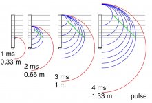
The MDDFL frontal acoustic load splits the incoming flat wave on multiple waveguides and re-emits them as spherical waves with delays between 1 and 2 milliseconds approximately. In the measurements made in the MDDHX135 prototype, the output measured responses from 400 Hz to 15 KHz for MDDFL and from 50 Hz to 1.5 KHz for MDDBL.
To use a compression driver it is necessary to adapt its emission to the input section of the MDDFL frontal acoustic load, I think they could work:
a small horn with the same output section of the MDDFL load,
an MDDFL load made with a bundle of thin copper pipes with a total section equal to the output diameter of the driver,
an MDDFL load made with several layers of alveolar polypropylene with 3 mm cells and with a total section equal to the driver's outlet diameter.
The emission is omnidirectional in a cylinder coaxial with the guides and with the height ranging from the lowest hole to the highest hole (green line). The output sound waves remain spherical as long as the wavelength is greater than the section of the single waveguide. If this limit is exceeded, the emission will no longer be omnidirectional but mainly directed upwards, the problem can be solved by using a greater number of waveguides with a smaller section.
The distribution of the lengths in a logarithmic series prevents resonances due to the distances between the exit holes, with the emission of hissing sounds.
The frequencies emitted by a compression driver are high enough not to create problems with the low frequency resonances of the L / 4 and L / 2 transmission lines.
Attachments
Log steps are necessary or I can cut pipe using smooth 3D spiral? Pipe could be slightly exponentially expanding? My delta wasp 2040 printer needs stepper replacement and after fixing I will print and test it out.
I see this mini version as a diffraction device - the log stepped tubes provide a load at the low frequency and the openings diffract sound at the high frequencies. I would think this scaled down version would work in a similar way as a Karlson tube - I am not sure if it would qualify as an MDD in this size. By the way, you might try the dual slot K-Tube as well (https://www.diyaudio.com/forums/mul...tube-1-compression-drivers-7.html#post6179069) - it is a very interesting HF device, IMHO better than a single slot due to the symmetrical dispersion pattern.
Log steps are necessary or I can cut pipe using smooth 3D spiral? Pipe could be slightly exponentially expanding? My delta wasp 2040 printer needs stepper replacement and after fixing I will print and test it out.
With a 3D printer you can perfectly adapt the section of the waveguides to the driver. In this post https://www.diyaudio.com/forums/full-range/341739-34c9-mdd-range-speakers-5.html#post5916484, they sent a render with the external spiral and the radial waveguides. At the exit of the guides the sound fronts would not be similar to spheres, I think they stretch on the axis aligned with the edge of the spiral. The omnidirectional effect would remain and also the delayed issue.
With the double K-Tube of pelanj, diffraction is used to make the emission omnidirectional, but with delays of less than a millisecond, I don't think we can perceive the MDD effect.
ABEC sims
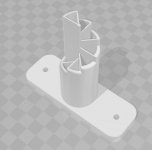
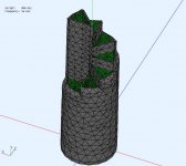
I've been asked by @jzgaja to run an ABEC sim for one of these MDD models. I used the model provided by @pelanj. Its a small version (8.5cm long) and meant to be driven from a 1inch compression driver. I was curious myself about how it works. If he prints it, it can be measured and compared to the sim model.
The model from @pelanj MDD Multi Delays Diffraction (Multi TL, omnidirectional, single drive, ...) had the base removed. It also has a small (2mm deep) chamber added between an ideal drive membrane and the 8 tubes.
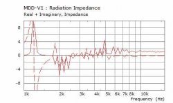
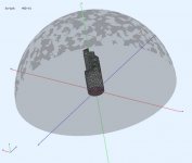
I'm not about the intended use, but the multiple openings suggest it might not radiant in a constant direction so I decided to use an observation hemisphere to capture radiation direction. The longest interior tube faces left (west). The radiation impedance suggests proper loading from ~2.6Khz.
I've been asked by @jzgaja to run an ABEC sim for one of these MDD models. I used the model provided by @pelanj. Its a small version (8.5cm long) and meant to be driven from a 1inch compression driver. I was curious myself about how it works. If he prints it, it can be measured and compared to the sim model.
The model from @pelanj MDD Multi Delays Diffraction (Multi TL, omnidirectional, single drive, ...) had the base removed. It also has a small (2mm deep) chamber added between an ideal drive membrane and the 8 tubes.
I'm not about the intended use, but the multiple openings suggest it might not radiant in a constant direction so I decided to use an observation hemisphere to capture radiation direction. The longest interior tube faces left (west). The radiation impedance suggests proper loading from ~2.6Khz.
Attachments
Last edited:
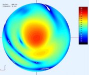
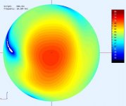
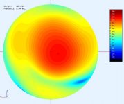
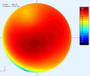
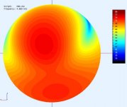
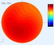
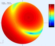
..... and now the observation fields (top view of the observation dome)
You can see that for lower freq the radiation is omni as the wavelength is much greater than the aperature perimeter. As the frequency rises (2Khz-8Khz), the radiation direction changes (lobes) and at high frequency (>8Khz) it becomes more directional.
The output SPL will varies because the radiation impedance varies. I've tried to show frequencies where the loading is similar to just show the radiation pattern.
It would be interesting to look at the pressures inside each interior tube and try to balance them.
.
Attachments
-
 MMD-V1-Hemi@16KHz.jpg33.2 KB · Views: 126
 -
 MMD-V1-Hemi@10K3Hz.jpg26.5 KB · Views: 108
 -
 MMD-V1-Hemi@8K6Hz.jpg25.3 KB · Views: 113
 -
 MMD-V1-Hemi@7K5Hz.jpg25.9 KB · Views: 112
 -
 MMD-V1-Hemi@5K8Hz.jpg26.2 KB · Views: 113
 -
 MMD-V1-Hemi@4K1Hz.jpg25.6 KB · Views: 117
 -
 MMD-V1-Hemi@3K4Hz.jpg23.6 KB · Views: 117
 -
 MMD-V1-Hemi@2K4Hz.jpg29.1 KB · Views: 109
 -
 MMD-V1-Hemi@1K85Hz.jpg29 KB · Views: 133
 -
 MMD-V1-Hemi@1K5Hz.jpg23.1 KB · Views: 142
Last edited:
Nice work DonVK..... and now the observation fields (top view of the observation dome)
You can see that for lower freq the radiation is omni as the wavelength is much greater than the aperature perimeter. As the frequency rises (2Khz-8Khz), the radiation direction changes (lobes) and at high frequency (>8Khz) it becomes more directional.
The output SPL will varies because the radiation impedance varies. I've tried to show frequencies where the loading is similar to just show the radiation pattern.
It would be interesting to look at the pressures inside each interior tube and try to balance them.
.
I would like to know how to use the ABEC simulator but for now I have to postpone.
I expected better results since in the last prototypes I come to reproduce 15 KHz, maybe I also measure the energy reflected by the walls.
I don't understand the directionality behavior. In the 5.8 KHz top view, the pressure is higher in the center (vertical emission) than in the edges (horizontal emission). By increasing the directionality with the frequency I expect that a decrease in the pressure on the edge corresponds to a further increase in the center. In the 16 KHz top view both the pressure in the center and on the edges decreases. In this simulation it seems that at high frequencies the sound energy is dissipated in turbulences generated by the geometry of the waveguides.
The first thing I would change in the model (if I knew how to do it) is the length of the waveguides and then I would try with circular and square sections.
Last edited:
I've been asked by @jzgaja to run an ABEC sim for one of these MDD models. I used the model provided by @pelanj. Its a small version (8.5cm long) and meant to be driven from a 1inch compression driver. I was curious myself about how it works. If he prints it, it can be measured and compared to the sim model.
The model from @pelanj MDD Multi Delays Diffraction (Multi TL, omnidirectional, single drive, ...) had the base removed. It also has a small (2mm deep) chamber added between an ideal drive membrane and the 8 tubes.
I'm not about the intended use, but the multiple openings suggest it might not radiant in a constant direction so I decided to use an observation hemisphere to capture radiation direction. The longest interior tube faces left (west). The radiation impedance suggests proper loading from ~2.6Khz.
If I could choose the first parameter to change in the simulation made by DonVK I would bring the space between the ideal membrane and the beginning of the waveguides from 2 mm to at least 10 mm. This activates the resonances of the waveguides open on both sides and the air could easily pass from one guide to the other.
I have not found in the description the radius of the hemisphere on which the SPL is calculated. With a radius greater than one meter, interference between sound fronts emitted by diffraction should be reduced.
Interesting. So maybe the HF we hear from the MDD is reflected from the ceiling. That might make sense, since the feel of the MDD sound is similar to FCUFS (floor coupled up firing speaker) that is discussed here: The Advantages of Floor Coupled Up-Firing Speakers I was experimenting with these some years ago.
What would be the best way to measure these? I have one printed. Maybe at 1 meter at ear height pointed at the listener and measure horizontal polars would be a good start? I can put on a Beyma CP385Nd.
What would be the best way to measure these? I have one printed. Maybe at 1 meter at ear height pointed at the listener and measure horizontal polars would be a good start? I can put on a Beyma CP385Nd.

Interesting. So maybe the HF we hear from the MDD is reflected from the ceiling. That might make sense, since the feel of the MDD sound is similar to FCUFS (floor coupled up firing speaker) that is discussed here: The Advantages of Floor Coupled Up-Firing Speakers I was experimenting with these some years ago.
What would be the best way to measure these? I have one printed. Maybe at 1 meter at ear height pointed at the listener and measure horizontal polars would be a good start? I can put on a Beyma CP385Nd.
Part of the HF arriving at the listening point are reflections from the ceiling. To get an idea of the proportion in the next few days if possible I will do an outdoor measurement that eliminates them.
For the measurement I would try to use reusable values in the simulation to understand if the model is in place or needs to be corrected.
measurements
Its relatively easy to measure the direct sound (MF+HF) in a room. It looks like you already have a UMIK and REW. You just need to setup the measurement properly.
I think you need 9 measurements, 8 radial (normal to each subtube) and 1 axial to determine the radiation pattern. The tube needs to be placed 1m off the floor, on a narrow stand, and isolated in the middle of the room. The mic needs to be attached to a boom, placed 1m off the ground and 1m from the MDD. You can use green painter tape to attach the mic to the boom (ie. could use a broom handle). Sound travels at 344m/s so we can time gate the measurement (1m = ~3ms) to exclude reflections.
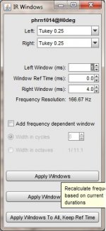
In REW : after you make a measurement sweep. Select [Tools]->[IR window] and change the popup box settings (see attached pic) then press [Apply Windows]. You can increase the Right Window to gradually include effects from reflections that occur later in time. You should also use vertical scale of 5dB/div so you can see the detail. I should also add that you should use a closed back driver if you want to see just the tube radiation.
Its relatively easy to measure the direct sound (MF+HF) in a room. It looks like you already have a UMIK and REW. You just need to setup the measurement properly.
I think you need 9 measurements, 8 radial (normal to each subtube) and 1 axial to determine the radiation pattern. The tube needs to be placed 1m off the floor, on a narrow stand, and isolated in the middle of the room. The mic needs to be attached to a boom, placed 1m off the ground and 1m from the MDD. You can use green painter tape to attach the mic to the boom (ie. could use a broom handle). Sound travels at 344m/s so we can time gate the measurement (1m = ~3ms) to exclude reflections.
In REW : after you make a measurement sweep. Select [Tools]->[IR window] and change the popup box settings (see attached pic) then press [Apply Windows]. You can increase the Right Window to gradually include effects from reflections that occur later in time. You should also use vertical scale of 5dB/div so you can see the detail. I should also add that you should use a closed back driver if you want to see just the tube radiation.
Attachments
Last edited:
Thanks for the indications, I will make these measurements with the next prototype that I am preparing.
Can I just rotate the tube not to move the mic? I will try to measure this tonight. Each tube + axial.
That's correct, just rotate the tube to point the subtube at the fixed mic. The mic should be aimed at the top of the subtube for radial measurements, and at the subtube bundle center for the axial measurement.
So I made some measurements. Instead of making pictures, here is the whole file: MDDTweeter.mdat - Google Drive
It is measured in room at 1 m distance, from the shortest tube to the longest, then the front. I rotated the driver 90 degrees so that the mic vs stand position in the room was not changed. The last measurement is just the driver without anything attached, pointed at the mic.
It looks like measurement nr. 6 has some kind of error, it is different from others.
Wow... that was fast @pelanj, thanks. It looks like you used a newer version of REW. I needed to register to get that newer version, so I'm waiting for the conf email. ........ 
A little more investigation. You are using V5.19, the same as me. For some reason I can only see the graphs provided in the "overlay" screen but not on the main screen. It's enough for me to do a comparison. Many thanks.
A little more investigation. You are using V5.19, the same as me. For some reason I can only see the graphs provided in the "overlay" screen but not on the main screen. It's enough for me to do a comparison. Many thanks.
Last edited:
JRE and REW
I also use version 5.19 but I can see all the graphs, the problem may be related to the JRE. In my pc the 1.8.0_181 32-bit on Windoows 10 version is installed.
Wow... that was fast @pelanj, thanks. It looks like you used a newer version of REW. I needed to register to get that newer version, so I'm waiting for the conf email. ........
A little more investigation. You are using V5.19, the same as me. For some reason I can only see the graphs provided in the "overlay" screen but not on the main screen. It's enough for me to do a comparison. Many thanks.
I also use version 5.19 but I can see all the graphs, the problem may be related to the JRE. In my pc the 1.8.0_181 32-bit on Windoows 10 version is installed.
So I made some measurements. Instead of making pictures, here is the whole file: MDDTweeter.mdat - Google Drive
It is measured in room at 1 m distance, from the shortest tube to the longest, then the front. I rotated the driver 90 degrees so that the mic vs stand position in the room was not changed. The last measurement is just the driver without anything attached, pointed at the mic.
It looks like measurement nr. 6 has some kind of error, it is different from others.
In addition to the measurements on the frontal acoustic load for tweeters pelanj has simultaneously published a post with the 3D printed version of the MDD 34c9 project.
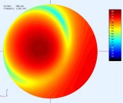
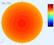
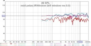
The pelanj prototype makes an HF unit omnidirectional. I think that listening can be perceived as a difference compared to the direct emission tweeter or with a horn as the frontal emission lobe widens to form a hemisphere. At the top, the sound pressure remains practically unchanged and is reflected by the ceiling (cyan line measured with direct emission, purple line measured with the guides). On the perimeter of the hemisphere the pressure is about 10 dB lower but uniform at 360 degrees as it must be in an omnidirectional diffuser (red line). It would be interesting to know the 90-degree attenuation of the driver mounted in direct emission.
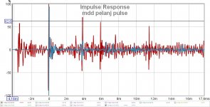
I set the parameter IRWindow-left-window with ms = 0.0 to compensate for an effect that can explain only those who know the algorithms used by the REW program. In the impulse response using the guides, delays are generated and the response begins in negative times (red line).
In this regard, the behavior of measure 6 is different also in the impulse response it seems that a slit at the base of the guides helps the algorithm to correctly calculate the offset.
The same phenomenon of impulse response with negative offset can be verified in all the REW files that I have published on the site.
Attachments
Last edited:
- Home
- Loudspeakers
- Planars & Exotics
- MDD Multi Delays Diffraction (Multi TL, omnidirectional, single drive, ...)