VituixCAD can do that. It just needs the horizontal and vertical measurements.Are there tools to generate cea2034 graphs from separate measurements? If e.g. REW could do that it would be nice.
I can quite easily generate and export data. If I don't have to do the calculations, that saves me some time and effort.
https://www.audiosciencereview.com/...ct-spinorama-cea2034-from-the-nfs-data.14141/
???
https://www.audiosciencereview.com/...s/20211124-octave-matlab-ppr-v1-0-zip.167722/
This appears to be the latest and most worked out version.
???
https://www.audiosciencereview.com/...s/20211124-octave-matlab-ppr-v1-0-zip.167722/
This appears to be the latest and most worked out version.
Last edited:
Tom, searching reading and absorbing is what I do daily. I can usually find things. Except for a few times. Like the original Thesis paper that Klippel based their system on. It is buried. Myself along with the truly smart people ( I'm not anywhere near these guys in my maths proficiency ) on the Audio Science thread tried for a few months to find that original paper. It is scrubbed off of the internet. But we did find a few alternate methods of doing the same thing by students that were not disciples of Herr Klippel. And those were available.
Last edited:
This has I think all the graphs a person would wish to have.You found it!
The spherical harmonics are always real, however each term in the series will be complex owing to the Hankel functions, which are always complex. The fitted coefficients would be complex in the most general case, but maybe real will work?. I investigated this and found that using complex coefficients made the HFs better fit the experimental data. At LFs there was little difference. Low frequencies have few modes in the sum (only one or two in many cases, with one often dominate) so their sensitivity to real versus complex would be much lower.I might have been using the wrong spherical harmonics (complex vs. real). It needs more investigation.
Last edited:
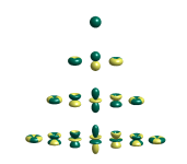
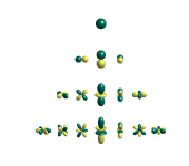
The left one is enshrined in the right one making it kind of redundant to add colors. The value of the function is simply how far that point is from the origin (r), and that's apparent from the right hand picture. This confused me when I first saw it (why two?), but then I figured out what I stated above.Here is a recreation of the image of spherical harmonics on wikipedia (colors: left the value, right the sign only):
View attachment 1467201View attachment 1467205
Do you mean the Weinreich paper? I have a copy. Somewhere.... for a few months to find that original paper. It is scrubbed off of the internet. But we did find a few alternate methods of doing the same thing by students that were not disciples of Herr Klippel. And those were available.
The spherical harmonics are always real, however each term in the series will be complex owing to the Hankel functions, which are always complex. The fitted coefficients would be complex in the most general case, but maybe real will work?. I investigated this and found that using complex coefficients made the HFs better fit the experimental data. At LFs there was little difference. Low frequencies have few modes in the sum (only one or two in many cases, with one often dominate) so their sensitivity to real versus complex would be much lower.
Complex:
Real:
https://docs.abinit.org/theory/spherical_harmonics/
As I have a lot to do, I'm not trying to fully understand every little detail. Others have identified the real spherical functions to be a good function set. For the processing, it's simply fitting. I expected them to look like in the Klippel docs/papers, but I found mine looked like the complex spherical functions, so I switched to real spherical functions.
I'm using complex coefficients, because that is what I get from the fit.
I could use some better measurements to improve the processing. For that I need to get it up and running again after my switch to wireless motion control.
Update:
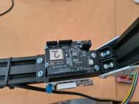
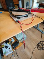
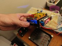
I'm designing and printing a support structure where all motion control electronics are mounted to. Everything (20V for servo, 5V usb for processing board) is powered from 20V and converted to 5V by the little board with the voltage display. Work in progress, which I plan to document along the way so others can build it too in the (near?) future.
I was looking into time gating the higher frequencies as done by Klippel and advocated recently by @gedlee over on ASR. I found an interesting function implemented by @mbrennwa.
@mbrennwa : Given this impulse response (which was made in a small room...)
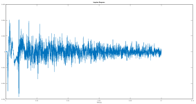
what parameters would you pass to the IR to FR with LF extension and why? I tried this:
[/CODE]
mataa_IR_to_FR_LFextend(hh,fs,0, 0.004, 0.1, 50, [],unit);
{/CODE]
The original code with just te IR to FR function can be seen here:
https://github.com/TomKamphuys/NTKSPH/blob/feature/3D/3D/read_nfs_measurements.m
ps. I still plan to do measurements in a larger space;
@mbrennwa : Given this impulse response (which was made in a small room...)

what parameters would you pass to the IR to FR with LF extension and why? I tried this:
[/CODE]
mataa_IR_to_FR_LFextend(hh,fs,0, 0.004, 0.1, 50, [],unit);
{/CODE]
The original code with just te IR to FR function can be seen here:
https://github.com/TomKamphuys/NTKSPH/blob/feature/3D/3D/read_nfs_measurements.m
ps. I still plan to do measurements in a larger space;
Hard to say from looking at the impulse response data alone. My idea was that if one knows the length of the anechoic time range (from the microphone/speaker/room geometry), this could be used to get the anechoic frequency response, and this could then be extended to lower frequencies by the echoic data (so the echoic range is the in-room response).
I'm having some troubles understanding the documentation:
% function [mag,phase,f,unit] = mataa_IR_to_FR_LFextend (h,t,t1,t2,t3,N,smooth_interval,unit);
%
% DESCRIPTION:
% Calculate frequency response (magnitude in dB and phase in degrees) of a loudspeaker with impulse response h(t) in two steps: first, the anechoic part (t < T0) is windowed and fourier transformed. Then, low-frequency bins in the range f0...1/T0 are added by using the part of the impulse response after T0 (the low-frequency response is therefore not anechoic).
%
% INPUT:
% h: impulse response (in volts)
% t: time coordinates of samples in h (vector, in seconds) or sampling rate of h (scalar, in Hz)
% t1, t2, t3: time ranges of the anechoic and the following echoic parts, relative to the first value in t. [t1,t2] is the time range used to calculate the anechoic frequency response, [t1,t3] the time range used to extend the frequency response towards lower frequencies (echoic part).
% N: number of frequency-response values to calculate in echoic frequency range
% smooth_interval (optional): if specified, the frequency response is smoothed over the octave interval smooth_interval.
% unit: see mataa_IR_to_FR
%
% OUTPUT:
% mag: magnitude of frequency response (in dB)
% phase: phase of frequency response (in degrees). This is the TOTAL phase including the 'excess phase' due to (possible) time delay of h(h). phase is unwrapped (i.e. it is not limited to +/-180 degrees, and there are no discontinuities at +/- 180 deg.)
% f: frequency coordinates of mag and phase
% unit: see mataa_IR_to_FR
Could you add t1, t2, t3 to the IR response? Is the time before t1 simply ignored? What is a good (default) value for N? Where does it depend on? And what does the code do conceptually?
Concept:
- Use the anechoic data in the time range [t1,t2] to calculate the anechoic part of the frequency response.
- [t1,t3] is the time range including both the anechoic and echoic response for calculation of the full frequency response.
- Determine the frequency frequency values for which to calculate the echoic low-frequency response:
N = number of frequency values
frequency range = [1/(t3-t1),1/(t2-t1)] - Stepwise extend the frequency response to the low-frequency values determined in step (3).
Why would you wish to add the echoic low-frequency response to the calculated anechoic response?
Not sure if this question is directed at me, but if it is: I was looking at different ways of measuring the frequency response of a speaker in a room, and I wanted to compare the anechoic/gated response with with an echoic measurement with smoothing applied. To this end I wanted to see what happens at the transition towards lower frequencies, which are not accessible by gating. This is why I made the mataa_IR_to_FR_LFextend(...) function for MATAA. I don't see (yet?) how this would be related to the Weinreich approach.
The easiest way to remove reflections is by time gating, which can be done for the higher frequencies (let's say >1khz).
For lower frequencies you need a longer signal and you inevitable measure the echo too. There the Sound Field Separation can take over the echo removal that was done by time gating for higher frequencies.
This echo removal is a separate feature of NFS, besides the capturing of the speakers radiation pattern in a set of coefficients and multiple methods to achieve the echo removal can be used.
- Home
- Design & Build
- Software Tools
- Klippel Near Field Scanner on a Shoestring
