
absolute air displacement is not relevant, according to my findings. it's always related to port radius.Ok, so I guess there are three major factors that affect port compression.
Exit strouhal, MSPN, and absolute air displacement?
no, that's just the case with straight tubes or very high curvature radius ports.In most designs, exit strouhal is the limiting factor.
furthermore, for very short ports (e.g. just a hole in the enclosure material) there is virtually no straight laminar air flow in the port. such ports are very prone to turbulent air flow.
there is one usual case in which ports tend to get very long: modern small woofers with low VAS that can (and should) be tuned low.
In order to get a low tuning frequency with a low enclosure volume the port needs to be very long (too long, thus needing PRs to be feasible).
In such a case a curved wall port can be ideal, because the smaller central diameter allows to make the port shorter and still have large opening diameters at the ends, to avoid turbulent air flow at exits.
But there is a limiting factor for this solution: once the displacement at the narrow middle section of the port gets very high, there will be uneven flow separation and turbulence and subsequent noise and compression.
of course. there are some ports that behave very badly because of shar edges. Then there are several ports that are simply far too small to be useful, but still provide good data for investigation.There is a lot of measurements to go through, I'm trying to make sense of them...
In some of your measurements, you seem to be getting significantly more compression at the same strouhal than I do. It looks like the compression/strohal varies quite a bit depending on the port design.
just for clairty: it's MPSN (for Mid Port Strouhal Number),In the post investigating MSPN, how did you separate MSPN effects from exit strouhal, given the correlation of mid vs end port area.
it's not possible to separate different effects. and there is of course a strong correlation between port exit strouhal number and mid port strouhal number.
I struggled quite long to try and get useful data, because it is so difficult to relate results of strongly varying tuning frequencies.
my " breakthrough" was relating parameters to the compression.
also have a look at the PDF showing all the port geometries in post #704.
by having a collection of very different port lengths, diameters and curvatures it was possible to guess what factor is most relevant for compression.
but several uncertainties still need some investigation.
Interesting! did you cover the entire inner port surface?Tried yesterday again lining of a reflex port with simple felt.
Yes - I can imagine that. The question is whether the uneven, fibrous material induces turbulent airflow at higher levels?Clearly absorbs emanation of mid frequencies audibly.
Hi, this was mighty useful, thank you!!if the port is around 63 cm long that would correspond to a 270 Hz wavelength:
speed of sound / (2 * tube length) = resonance frequency
340 m/s / (2 * 0,63 m) = 340 / 1,26 s = 270 1/s = 270 Hz
depending on the distance between port exit and driver that will result in a deep notch, similar to the one you measured.
a deep notch in frequency response always translates into a sudden phase shift. the two are inherently connected (considering a minimum phase system).
even a very deep notch is usually not very audible and most importantly, this notch will not be there (or not as trong) in a real listening situation, including reflected sound. There might however be a problem if there is a narrow peak of total sound energy at 270 Hz.
you could measure that with the microphone at your listening spot and with no or long gating times.
It's not really that important to provide both graphs - in other words you can look at either graph and know what's going on - but response graphs are easier to interpret for me 🙂
you can see the effect of a port resonance for the total response in my measurements here.
Indeed I have port straight behind the driver, as in your linked post, later I will sketch speaker internals just to be easy to see.
In room, both speakers on and in listening position (or about it, we walk a lot 🙂, the 270Hz distortion is pretty much gone as you suggested it would probably. Tons of other room elements come in to mess the graph up completely, but that 270 Hz thing is not that visible any more, if at all, just like you said....
This is in room, stereo driven in the roughly listening place:
Calculations above show first resonance, but it has also harmonics at 2x, 3x etc. frequencies. Can the math tell the relative strength of harmonics? Overload turbulence is more like noise, but is it mostly at resonance F?
As we know and have seen in measurements, port resonance and noise can be problematic with 2-way speakers. If port is wide and/or on the front baffle, typical problems can be seen in even at low spl in frontal frequency response, and best in 360deg spinorama.
As we know and have seen in measurements, port resonance and noise can be problematic with 2-way speakers. If port is wide and/or on the front baffle, typical problems can be seen in even at low spl in frontal frequency response, and best in 360deg spinorama.
only if there are sharp edges and/or for very long ports with low flare rate.but is it mostly at resonance F
usually the resonance strength is reduced with higher harmonic number. you can simulate the port resonances (but not the resonance chuffing or turbulent noise) with hornresp. so I guess there is a mathematic formula behind it!Can the math tell the relative strength of harmonics?
EDIT: if you activate enclosure resonance masking and only show the port output you can see the isolated port resonances, here with a 63 cm port (disregard helmholtz tuning):

Last edited:
There is probably something wrong with my calculations.1)
the "91 mm" port using the small SICA box (tuned to 77 Hz) and the bigger MONACOR box (tuned to 41,5 Hz).
Both the graphs for SN and MPSN are very similar. The MONACOR speaker is slightly better, as far as I have observed because of lower tuning.
View attachment 1342101
At the 2.83V measurement point, in the 41.5 Hz tuned box with the 91mm long port, the chart reads strouhal ~1.3.
When i try to calculate the same value, I get:
Air displacement: (19/(41,5*2*pi)) = 0,075 m or 7.5cm
Port exit area: (from drawing) 4,4*2,46^2 = 27 cm²
port exit radius: sqrt(27/pi) = 2,9 cm
2,9/7,5 = 0,4
So I think I'm doing something wrong...
it was black felt 1mm thick or 1.5mmInteresting! did you cover the entire inner port surface?
Yes - I can imagine that. The question is whether the uneven, fibrous material induces turbulent airflow at higher levels?
of this type and I covered the reflex port completely with it fixing with glue
it only sounds better because I wanted to tune the reflex lower, too. As side effect.
you cannot use the air velocity of the middle port section.Air displacement: (19/(41,5*2*pi)) = 0,075 m or 7.5cm
you would need to relate it to the mouth surface first:
velocity at mouth = mid-velocity * Amin / Amouth
in my case this is 4,57 m/s translating into 1,75 cm displacement and a corresponding strouhal number of 1,3.
that's the interesting thing: the port diameter is proportional to the radius, but the velocity will decrease by the square of diameter (or radius), because the velocity is inverse to the surface area.
so changing the port diameter just slightly will massively change the strouhal number (and the MPSN).
there is something wrong with your calculation... or my drawing is misleading.Port exit area: (from drawing) 4,4*2,46^2 = 27 cm²
the effective port mouth diameter is 48 mm, radius is 2,4 cm.
Last edited:
Calculations above show first resonance, but it has also harmonics at 2x, 3x etc. frequencies. Can the math tell the relative strength of harmonics?
Sound is a linear perturbation about mean fluid conditions. Linear means there are no harmonics. To predict sound harmonics we need to consider more than just the linear wave equation which can be done in a number of ways. Unfortunately what we consider has to be nonlinear and to include motions involving at least vorticity as well as sound which means CAA/CFD rather than linear acoustic BEM/FEM.
The most cost effective appraoch for fluid speeds before the onset of turbulence (i.e. only discrete tonal frequencies) is likely to be aeroacoustic harmonic balance. This effectively requires a steady state CAA/CFD simulation to be performed for the fundamental frequency and repeated with slightly different terms for the first few harmonics. It also requires the use of a nonlinear model for the driver which, as Tenson pointed out earlier, much of the data for which is starting to become available for some drivers like those from Dayton. If the software can be sorted out a reasonable set of frequencies is likely to be doable with a good desktop though it might take a few overnight runs.
When turbulence and chuffing starts it is very unlikely at such low Reynolds numbers a steady state turbulence model will be able to represent the stresses in a meaningful way and so the full unsteady Navier-Stokes equations will need to be solved through time. This not only becomes computationally large but there will be numerical problems to do with scale at such low Mach numbers. Performing a frequency sweep (i..e. like an experiment) is likely to require a fair few overnight runs on a good desktop machine and will be pushing what is viable at home. Of course one can hire time on a remote High Performance Cluster (HPC) easily these days but the cost will likely be pushing that of a good desktop after one or two runs.
Overload turbulence is more like noise, but is it mostly at resonance F?
The velocity of the flow needs to be high for turbulence to begin and the highest velocities occurs at or near the resonant frequency. There seems to be some confusion in this thread about what is turbulent flow and what is unsteady laminar flow.
Thank you! I have corrected all my calculations. Again!you cannot use the air velocity of the middle port section.
you would need to relate it to the mouth surface first:
velocity at mouth = mid-velocity * Amin / Amouth
in my case this is 4,57 m/s translating into 1,75 cm displacement and a corresponding strouhal number of 1,3.
that's the interesting thing: the port diameter is proportional to the radius, but the velocity will decrease by the square of diameter (or radius), because the velocity is inverse to the surface area.
so changing the port diameter just slightly will massively change the strouhal number (and the MPSN).
there is something wrong with your calculation... or my drawing is misleading.
the effective port mouth diameter is 48 mm, radius is 2,4 cm.
I've added some of your ports, and two subwoofers from data-bass to my spreadsheet, 21SW152 25Hz and BMS 18n862 compact.
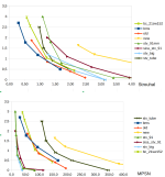
I wanted to compare port velocity and strouhal number, as a predictor of port compression.
Note that I have not attempted to remove thermal compression from these graphs.
As you can see, in the >1 strouhal range, it is a good predictor for port compression if my new port and stv:s 91mm port in both enclosures are excluded
Here is mid port air velocity. Good predictor for compression if we exclude your tube port, the 91mm port in 41,5Hz tuned enclosure and bms18n862 port from data-bass.
So what about the exclusions?
For the strouhal number chart, I think that my new port and the 91mm port in the sica enclosure simply reach too high mid port air velocity to benefit from the large vent opening. The 91mm port in the 41,5Hz enclousure, is probably limited my MPSR.
If we look at the air velocity chart. I think that stv tube port, and the BMS port is limited by strouhal number. stv:s 91mm port is once again limited by MPSR.
I looked through your charts again, and I could not find a port that compressed less than 1 db at 30 m/s, except the SONY woofer that sometimes had backwards compression. So it looks like port velocity does matter, although another explanation is that might just have messed up some formulas again...
Attachments
As expected, I made another mistake, the stv tube port was affected by an input error in my previous post. Fortunately, the other ports were unaffected.
I'll re-upload the charts. I have also added your 3d_big port to the charts.

The 3d_big port does very well, compared to the strohal value...

And MPSN...

Also good air velocity performance, but it does not completely outdo the other ports in this regard.
Here is some analysis on the limiting factors for port performance:

The chart displays mid port velocitty, strouhal and MPSN at 1,5 db compression (linear interpolation used to get values at "exactly" 1,5 db) and some speculation on what's causing the compression.
Limits:
Strohal: <1.0 red; <1.4 orange
MSPN: <20 red
Velocity: >30 red; >25 orange
I'll re-upload the charts. I have also added your 3d_big port to the charts.
The 3d_big port does very well, compared to the strohal value...
And MPSN...
Also good air velocity performance, but it does not completely outdo the other ports in this regard.
Here is some analysis on the limiting factors for port performance:
The chart displays mid port velocitty, strouhal and MPSN at 1,5 db compression (linear interpolation used to get values at "exactly" 1,5 db) and some speculation on what's causing the compression.
Limits:
Strohal: <1.0 red; <1.4 orange
MSPN: <20 red
Velocity: >30 red; >25 orange
Thank you once more for the effort you put into this!
I appreciate it very much, as it proves my explanation attempts seem sensible!
In short you are coming to similar or the same conclusions i described in post #704.
By keeping the flares low (in other words: keeping NFR Normalzed Flare Rate low) the compression effect when reaching low strouhal numbers for the port mouth is very mild.
I would conclude that for subwoofer ports or 3-way systems, where the port length is not very critical regarding port resonance, it's best to make a low (0.15-0.3) NFR port.
For 2-way or full range systems without high SPL requirenents a higher NFR port (0.5) is probably easier to implement.
The advantage of a NFR=0.5-port is it's short length (higher resonance frequency and generally less susceptibility for resonance) and the very low compression at reasonable levels.
I appreciate it very much, as it proves my explanation attempts seem sensible!
In short you are coming to similar or the same conclusions i described in post #704.
Yes, indeed.The 3d_big port does very well, compared to the strohal value...
By keeping the flares low (in other words: keeping NFR Normalzed Flare Rate low) the compression effect when reaching low strouhal numbers for the port mouth is very mild.
I would conclude that for subwoofer ports or 3-way systems, where the port length is not very critical regarding port resonance, it's best to make a low (0.15-0.3) NFR port.
For 2-way or full range systems without high SPL requirenents a higher NFR port (0.5) is probably easier to implement.
The advantage of a NFR=0.5-port is it's short length (higher resonance frequency and generally less susceptibility for resonance) and the very low compression at reasonable levels.
Thank you stv for your measurments and explanations.
I've been messing around with the port measurement data some more, and attempted to create a model that predicts port compression (or, I did, but I'm not sure it works yet, so I'll go with "attempted").

Y axis: Measured compression in decibels
X axis: Predicted compression in decibels
The blue dots are all the ports included in my previous posts, I used that data to create the model ("calibration").
The progr_big (stv) and B&C 21ds115 X21 was added after the model was created, to see if the model predictions work for ports not included in the calibration data. I should have added a few more, but I was a little tired of entering data, I can say it worked for those ports though.

Correlation coefficents for different predictors of compression, and measured compression.
The (cal) coefficents only use calibration data for the model.
As you can see, the correlation for the model actually increased after adding the progr_big and data-bass X21 ports, which is a good sign, but I might just have been lucky.

Yellow voltage = possible thermal compression
I used U^2/Znom > 0,7*AES for the large speakers and U^2/Znom > 0,5*RMS for the monacor driver. (I guessed you had the 4 ohm version, could be wrong)
I intend to upload the spreadsheet here after cleaning it up. 🙂
The model:
EAPV * (10*LOG(10*WACR-10))^-1 = predicted compression in decibels
Basically, the log function estimates the (compression/air velocity) slope based on a weighted area/circumference ratio of the port.
Acronyms:
EAPV (Equivalent Average Port Velocity):
Equivalent velocity in a straight tube that (according to my guesses) causes the same resistance. This does not include turbulence at the ends.
I used the online graphing calculator desmos to calculate an EAPV ratio for ports with large flares.
Method:
Created a function for port area vs distance from the middle of the port (half length). I'll refer to this as f(x) (Note: Only works for symmetrical ports with minimum radius in the middle)
created another function based on f.
g(x) = f(0) / f(x)
This should give us the air velocity ratio between x cm from center and peak velocity.
If, for instance g(6)=0,7 and peak air velocity is 20 m/s, port velocity 6 cm away from the middle of the port should be 20*0,7 = 14 m/s.
Calculating the area under the curve (between port ends) and dividing by port length should give us the (average/peak) air velocity ratio inside the port.
However, air resistance is air velocity squared, 1 cm length with 30 m/s most likely causes more resistance than 3 cm with 10 m/s.
So I used (g(x))²
Then calculated the area under the curve, and divided the result with port length, I'll call this the air resistance ratio.
Then we have: air resistance ratio * peak velocity = EAPV.
WACR (Weighted area circumference ratio):
I calculated average port circumference (AVGC), average cross sectional area (AVGA), and exit cross sectional area (EA) for all ports. I averaged end and average area and divided by average circuference.
WACR = ((AVGA+EA)/(2*AVGC)
As the model is based on area at different sections of the port, very abrupt end flares will probably mess up the predictions. Ports with an average flare width/lengtht ratio < 1 are included in the dataset, and should be fine.
I've been messing around with the port measurement data some more, and attempted to create a model that predicts port compression (or, I did, but I'm not sure it works yet, so I'll go with "attempted").
Y axis: Measured compression in decibels
X axis: Predicted compression in decibels
The blue dots are all the ports included in my previous posts, I used that data to create the model ("calibration").
The progr_big (stv) and B&C 21ds115 X21 was added after the model was created, to see if the model predictions work for ports not included in the calibration data. I should have added a few more, but I was a little tired of entering data, I can say it worked for those ports though.
Correlation coefficents for different predictors of compression, and measured compression.
The (cal) coefficents only use calibration data for the model.
As you can see, the correlation for the model actually increased after adding the progr_big and data-bass X21 ports, which is a good sign, but I might just have been lucky.
Yellow voltage = possible thermal compression
I used U^2/Znom > 0,7*AES for the large speakers and U^2/Znom > 0,5*RMS for the monacor driver. (I guessed you had the 4 ohm version, could be wrong)
I intend to upload the spreadsheet here after cleaning it up. 🙂
The model:
EAPV * (10*LOG(10*WACR-10))^-1 = predicted compression in decibels
Basically, the log function estimates the (compression/air velocity) slope based on a weighted area/circumference ratio of the port.
Acronyms:
EAPV (Equivalent Average Port Velocity):
Equivalent velocity in a straight tube that (according to my guesses) causes the same resistance. This does not include turbulence at the ends.
I used the online graphing calculator desmos to calculate an EAPV ratio for ports with large flares.
Method:
Created a function for port area vs distance from the middle of the port (half length). I'll refer to this as f(x) (Note: Only works for symmetrical ports with minimum radius in the middle)
created another function based on f.
g(x) = f(0) / f(x)
This should give us the air velocity ratio between x cm from center and peak velocity.
If, for instance g(6)=0,7 and peak air velocity is 20 m/s, port velocity 6 cm away from the middle of the port should be 20*0,7 = 14 m/s.
Calculating the area under the curve (between port ends) and dividing by port length should give us the (average/peak) air velocity ratio inside the port.
However, air resistance is air velocity squared, 1 cm length with 30 m/s most likely causes more resistance than 3 cm with 10 m/s.
So I used (g(x))²
Then calculated the area under the curve, and divided the result with port length, I'll call this the air resistance ratio.
Then we have: air resistance ratio * peak velocity = EAPV.
WACR (Weighted area circumference ratio):
I calculated average port circumference (AVGC), average cross sectional area (AVGA), and exit cross sectional area (EA) for all ports. I averaged end and average area and divided by average circuference.
WACR = ((AVGA+EA)/(2*AVGC)
As the model is based on area at different sections of the port, very abrupt end flares will probably mess up the predictions. Ports with an average flare width/lengtht ratio < 1 are included in the dataset, and should be fine.
I had apparently calculated the circumference for all the round ports as pi*r instead of pi*d.
I have now fixed that, and recalibrated the model. I did not use the last two ports for calibration, to keep raw data the same.

Correct input data gives you better predictions!

The new, adjusted formula is
(EAPV-4)*(10*LOG(7*WACR-3,5))^-1
Results below zero are set to zero.
I have uploaded the spreadsheet.
I have now fixed that, and recalibrated the model. I did not use the last two ports for calibration, to keep raw data the same.
Correct input data gives you better predictions!
The new, adjusted formula is
(EAPV-4)*(10*LOG(7*WACR-3,5))^-1
Results below zero are set to zero.
I have uploaded the spreadsheet.
I've tweaked the model a bit, and made a desmos link so people can try it.
For "tube" ports with circular flares:https://www.desmos.com/calculator/alrsqx2a36
For NFR ports: https://www.desmos.com/calculator/qv9sjpvff7
x= peak air velocity (m/s)
y= compression (db)
I've found that the model becomes unreliable with the combination high flare rate and high velocity, so it will not make predictions when
(Peak Velocity (m/s) - EAPV (m/s))/ port length (cm) exceeds 0.9.
I'll explain this, and some other stuff in more detail later...
Sorry, I keep making mistakes. There are some errors in the "tube" port desmos model. The NFR model does not seem to be affected.
I have fixed it, here is the new link:
Tube, circular flare: https://www.desmos.com/calculator/xrizx1eu4z
This one should be ok, as always.
I have some trouble keeping track of everything, but I'm getting more optimistic this model might actually be working...
I have fixed it, here is the new link:
Tube, circular flare: https://www.desmos.com/calculator/xrizx1eu4z
This one should be ok, as always.
I have some trouble keeping track of everything, but I'm getting more optimistic this model might actually be working...
Don't apologize, this whole thread is a series of mistakes with corrections ...Sorry, I keep making mistakes.
I keep trying to follow your very promising formulas for the estimation of compression, but I'll need even more time.
I am glad you invest your knowledge, because for me that would be very difficult or impossible!
You are right, by the way, the monacor woofer is the 4 ohm variant.
Let me know if my collection of data would be useful for you in excel fomat. I can send it to you, I'll just have to re-organize it, it's quite a mess at the moment.
Thank you and yes, your collection of data would be very useful to check the model.
I'm going to make a post that explains everything in more detail, I need some time, but I can hopefully get it done in a week or so.
Please ask if you have any questions, it would make it easier to choose what parts should be the focus of the explanation post, and most likely, I'll be able to answer them before I'm done with the post.
- Home
- Loudspeakers
- Multi-Way
- Investigating port resonance absorbers and port geometries