traderbam said:
This diagram is what I define to be a GNF system. So based on your latest comment to Jan that HEC topology is different from GNF, and based on your earlier paper "why error correction is conceptually different from negative feedback?", I suppose I can only draw the conclusion that your definition of GNF must be different from mine.
If it is my definition of a GNF system that is wrong, then I must change it.
Hi Brian,
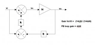
I think I can agree with you. It is a GNF system that includes a PFB segment of gain in its forward path. That PFB segment of gain will typically have a gain greater than unity. The b path closes the loop around this with GNF. Things get interesting as in the sense of HEC when a goes to unity, providing the "infinite" forward loop gain. I think this is the essence of the NFB view of HEC.
Cheers,
Bob
traderbam said:
Wow. I must say I am surprised at you, Rodolfo, for introducing this wild sophistry into the discussion. For goodess sake...comparing it to wave duality!
This is a very simple system that is objectively describable using simple algebra. There are no quantum uncertainties at work. I think it is quite simple...but perhaps I am a genius like the late Richard Feynman.
The purpose of objective analysis is to keep us humble and to stop us from believing what we want to believe, rather than what is real. Jan's post tag-line quote from CH exemplifies this.
😎


wave/particle isn't quantum uncertainty.
it's the same house, just looking through a different window.
i think the example is great.
traderbam said:
Suppose I were to do the opposite of what you suggest and separate the inner loop from the input summer...it can have a separate summer to itself (the input summer feeds into the new summer). Now, the input summer is exactly like Black's.
According to your definition, is this HEC or is this GNF?
Of course you can, forward gain then becomes infinite (under ideal cancellation conditions).
This I can tell without sorting the actual math because, correctly done it must end in the same result. Left as excercise.
Minutiae aside, this approach loses sight of what matters, that is the EC as a topology, extracts the *net error* and uses it for correction (that's why I assume it was called Error Correction in the first place).
Rodolfo
Bob Cordell said:
....
I also like that you noted that real-world implementation delays and imperfections limit the distortion reduction achievable with both HEC and NFB. We should also throw feedforward error correction in there as well....
This is why I guess EC elicits heated debate when applied in "real time" within an analoge context.
Unless some analog guru comes out with a very clever summing node design that ends up making a better integrator (closing the inner loop) than the best Op Amp, then I am afraid there is not much to be expected in terms of performance.
Of course some schemes like your own local EC output stage are worth considering when properly executed, just as other schemes resorting to multiple tandem NFB stages tailored for performance and weak GNF may in some cases yield better performance than the more traditional Op Amp type design.
But if the real time on the spot correction is replaced with a quasi static precorrection based on the error extraction, then all the stability issues disappear as well as any similarity with NFB.
It remains to be seen how practical this approach may prove.
Rodolfo
HEC is positive feedback on demand
Here is a version of the feedback-on-demand view of HEC.
With a slight chuckle, I am throwing this into the mix just to create more confusion.
HEC is actually a POSITIVE feedback system. The voltage across the output stage, from input to output, is fed back as an error and added to the input signal to the output stage. It is added in such a way that increased drop across the output stage is added in-phase with the signal to the input of the output stage. Thus, if the output stage has a gain of 0.9, then positive feedback with a loop gain factor of about 0.1 is fed back to the input. This results in a slight gain enhancement to the otherwise near-unity-gain system.
Now realize that MOSFET output stage distortion is largely a result of changes in output stage transconductance as a function of output current. Thus the output stage can be modeled as a perfect unity gain buffer followed by a variable resistor – one whose resistance depends on the current flowing. It is the voltage across this resistor that is fed back and added to the input of the output stage.
The gain of the output stage is just that of the resistor divider formed by this varying output resistance against the load resistance.
We are now free to swap the load resistance and the output resistor modeling the output stage, placing the latter at the ground end. We now need only take the single-ended voltage from this resistor and feed it back. Again, it is fed back as positive feedback. It is positive feedback whose amount is varied depending on the resistance of the variable resistor modeling the output stage. The voltage across the now-floating load resistor is still the same, and is what it should be. We thus have a simple positive feedback system whose loop gain is dependent upon the value of the nonlinear resistance. Notice that if this feedback goes to zero, we are left with the simple near-unity-gain amplifier.
Notice also that this is extremely reminiscent of the old tube amplifiers that had a variable damping factor feature, where the damping factor could be adjusted upward or downward with feedback that was positive or negative, and where the feedback was sensed by a small resistor in series with the return of the loudspeaker. Indeed, some have also used a feature like this to adjust the effective Q of a loudspeaker downward by feeding it with what amounted to a negative resistance to wipe out a portion of the voice coil DCR.
It is also interesting to realize that the primary form of frequency compensation in the Cordell version of the HEC circuit acts to reduce the feedback of the error signal at high frequencies, as opposed to putting a pole in the forward path of the system. At the same time, it is also fair to note that the secondary compensation, the small capacitor to ground in the emitter circuit of the error differencing amplifier, acts to interfere with the positive feedback loop so as to reduce its gain from theoretically infinity down to a smaller very finite value at high frequencies.
I am not claiming that this view of HEC (positive feedback on demand) is one that provides good insight on stability. Indeed, it may provide a misleading view on stability. For example, if the loop-gain-on-demand is so small, be it positive or negative, how can we possibly get into stability trouble. Maybe I am missing something here. I’m just throwing this all out as a brain teaser.
Cheers,
Bob
myhrrhleine said:wave/particle isn't quantum uncertainty.
it's the same house, just looking through a different window.
i think the example is great.
There are some excellent Feynman videos about this topic on YouTube. I recommend them.
I don't like the analogy for two reasons. 1) With photons you can use the particle model and find it fails one test, and then you can use the wave model and find it fails another test. Therefore, neither model is correct. With HEC we have a model that passes all tests. But with HEC we have descriptive claims that either contradict or are unsupported by the mathematical model and fail the tests. 2) Comparing the HEC lack of comprehension to that of light gives the HEC lack of comprehension an undeserved legitimacy and credibility.
I suppose the stubbornness and egos that get involved in the two subjects may be analogous.

ingrast said:
Of course you can, forward gain then becomes infinite (under ideal cancellation conditions).
This I can tell without sorting the actual math because, correctly done it must end in the same result. Left as excercise.
Minutiae aside, this approach loses sight of what matters, that is the EC as a topology, extracts the *net error* and uses it for correction (that's why I assume it was called Error Correction in the first place).
Rodolfo
Well, you didn't answer my question. The way you talk, it seems to me that your real focus is on a specific implementation of a practical summer; a subtractor/integrator combo. That is novel and interesting, but I don't think it defines a functional difference with any other NFB system.
As for extracting the "net error", this is not unique to HEC either. This is how servos are often configured and servo-assist circuits. I would not call a servo an EC or a HEC just because it adds the difference between input and output to the input. This is not distinguishing. Using a PFB to generate gain is unusual but not original - this technique has been used in valve amps before I was born.
So this leaves me and my equations with no clear differentiator for HEC. For now, my analysis shows HEC to belong to the general class of NFB control systems, within the servo sub-category, with the unusual (but not essential) facility of a PFB nested loop to generate excess gain.
The reason I say a "tunable" PFB loop is not essential is because an equally ideal integrator can be made in practice using a transconductance stage and a capacitor. Nevertheless, the HEC topology makes a PFB integrator easier to implement.
As for hypotheses...
If I can help anyone objectively analyse a hypothesis, I'll be happy to try. But you need to define clearly what the hypothesis is, and its really up to you to let go of it if it is wrong or unverifiable.
"NFB on demand" - I still don't understand the definition.
Brian's Error Correction
I'm going to take Bob's lead and throw another cat into the pigeon coup just for fun.
Here's my answer to HEC. Let's call it Brian's EC or BEC for short. I have incorporated the "wow" elements: only the error in the output is fed to the input, if the feedback signal to the input is cut the circuit becomes a simple follower. If you want infinite dc gain you can make K a perfect integrator (PFB or otherwise).
😎
PS: it's really just a servo circuit.
Attachments
traderbam said:
... For now, my analysis shows HEC to belong to the general class of NFB control systems, within the servo sub-category, ..
Turning the argument around, then you may as well dismiss all forms of servo systems insofar as they are equivalent to single loop NFB. Is that what you want?
On the other hand, if what you want is to make me admit HEC is NFB where the error instead of the signal is what is fed back, well, this is what I've been saying all the time.
Rodolfo
PS This is as far as I will go on this issue, there are more interesting matters to pursue/discuss than a taxonomy of feedback systems.
blind spot?
Hi Jan,
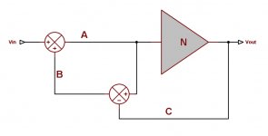
If I understand you correctly, you are saying that the only way to get insight in the amount of error reduction is by cutting the loop at point A, right?
Well, Brian's method (and mine) -cutting the loop at C- also predicts to which extent the error will be reduced. If the DC loop gain is 40dB, for example, the error will be reduced to 1% of its original value. Another example: suppose the loop gain at 60kHz is 30dB, then the 3rd harmonic of 20kHz will be reduced by a factor of 31.6, etc.
Please correct me if I misunderstood your point.
Regards,
Edmond.
janneman said:[snip]
I think we agree that cutting it either at say, A or at C, gives different views and different attributes of that particular loop we thus created. I agree that cutting it at C does expose the infinite gain loop.
Cutting it at A, for example, exposes other attributes. For example, it shows that the error reduction at low frequencies is limited to the accuracy of 'a' (and the input summer), in that an accuracy of 1% gives you a max error reduction of 40dB.
As another example, it shows you that if you want this 40dB reduction up to frequency fe, your 'a' should have its -3dB frequency at least 2 decades above fe.
These are attributes that can readily be verified in calculations or in actual hardware, and confirm teh results of analyzing the loop in that way. Surely the purpose of analyzing the loop is to gain insight in how the actual system behaves? I don't see how analyzing the loop as proposed by Brian, while possibly interesting as an academic exercise, tells me how my system will behave, with the examples shown as well as in other ways. Maybe that is my blind spot?
Jan Didden
Hi Jan,
If I understand you correctly, you are saying that the only way to get insight in the amount of error reduction is by cutting the loop at point A, right?
Well, Brian's method (and mine) -cutting the loop at C- also predicts to which extent the error will be reduced. If the DC loop gain is 40dB, for example, the error will be reduced to 1% of its original value. Another example: suppose the loop gain at 60kHz is 30dB, then the 3rd harmonic of 20kHz will be reduced by a factor of 31.6, etc.
Please correct me if I misunderstood your point.
Regards,
Edmond.
Re: blind spot?
Hello Edmond,
We xposted. I know which picture you referred to.
Interesting point. My point was that when you cut the loop at C instead of A you would get different values for loop gain and feedback. What you are saying now, if I understand you correctly, is that this may be the case, but still the final result, as far as the relationship between Vo and Vi, is identical.
I think we knew this already but maybe didn't give it enough attention: Brian's view and mine both lead to the same clg.
Maybe in the final analysis that is what Bob calls the different views: each view has its own, different, set of loop gain and feedback factor, but in each case the resulting clg behaviour is identical.
Speculating: looking ahead to an analysis where each element (K, a, b) is a function of the complex variable s, how would that manifest itself in the different views?
I wish I'd gone to university 40 years ago 😱
Jan Didden
Edmond Stuart said:
Hi Jan,
If I understand you correctly, you are saying that the only way to get insight in the amount of error reduction is by cutting the loop at point A, right?
Well, Brian's method (and mine) -cutting the loop at C- also predicts to which extent the error will be reduced. If the DC loop gain is 40dB, for example, the error will be reduced to 1% of its original value. Another example: suppose the loop gain at 60kHz is 30dB, then the 3rd harmonic of 20kHz will be reduced by a factor of 31.6, etc.
Please correct me if I misunderstood your point.
Regards,
Edmond.
Hello Edmond,
We xposted. I know which picture you referred to.
Interesting point. My point was that when you cut the loop at C instead of A you would get different values for loop gain and feedback. What you are saying now, if I understand you correctly, is that this may be the case, but still the final result, as far as the relationship between Vo and Vi, is identical.
I think we knew this already but maybe didn't give it enough attention: Brian's view and mine both lead to the same clg.
Maybe in the final analysis that is what Bob calls the different views: each view has its own, different, set of loop gain and feedback factor, but in each case the resulting clg behaviour is identical.
Speculating: looking ahead to an analysis where each element (K, a, b) is a function of the complex variable s, how would that manifest itself in the different views?
I wish I'd gone to university 40 years ago 😱
Jan Didden
Re: Re: blind spot?
Hi Jan,
I'm glad we agree on those points.
Graduated or not, doing such analysis by hand is always cumbersome. Let a simulator do the dirty job.
Much faster, less errors.
Regards,
Edmond.
janneman said:Hello Edmond,
We xposted. I know which picture you referred to.
Interesting point. My point was that when you cut the loop at C instead of A you would get different values for loop gain and feedback. What you are saying now, if I understand you correctly, is that this may be the case, but still the final result, as far as the relationship between Vo and Vi, is identical.
I think we knew this already but maybe didn't give it enough attention: Brian's view and mine both lead to the same clg.
Maybe in the final analysis that is what Bob calls the different views: each view has its own, different, set of loop gain and feedback factor, but in each case the resulting clg behaviour is identical.
Hi Jan,
I'm glad we agree on those points.
Speculating: looking ahead to an analysis where each element (K, a, b) is a function of the complex variable s, how would that manifest itself in the different views?
I wish I'd gone to university 40 years ago 😱
Jan Didden
Graduated or not, doing such analysis by hand is always cumbersome. Let a simulator do the dirty job.
Much faster, less errors.
Regards,
Edmond.
Re: Re: Re: blind spot?
For this, I prefer Mathcad. No hassle with models 😉
Can you agree to my transformation to situation C in my earlier post?
Jan Didden
Edmond Stuart said:[snip] Let a simulator do the dirty job.
Much faster, less errors.
Regards,
Edmond.
For this, I prefer Mathcad. No hassle with models 😉
Can you agree to my transformation to situation C in my earlier post?
Jan Didden
I guess you mean C in post 3611. Well, to a certain extent. See my post 3564.
Regards,
Edmond.
Regards,
Edmond.
Re: New President Obama
Hi Brian,
Yes, I think the great majority of us are hopefully optimistic, even a great many of those who voted the other way. So far, so good!
Cheers,
Bob
traderbam said:Way to go America!!!


Hi Brian,
Yes, I think the great majority of us are hopefully optimistic, even a great many of those who voted the other way. So far, so good!
Cheers,
Bob
/OT
Yes I know Edmond, politics is out-of-bounds.
Yet: my congratulations to the US of A. The son of a man who couldn't order a cup of coffee in a restaurant due to his race, is now President.
Indeed, as Diana Feinstein said, the victory of ballot over bullet.
/OT off
Jan Didden
Yes I know Edmond, politics is out-of-bounds.
Yet: my congratulations to the US of A. The son of a man who couldn't order a cup of coffee in a restaurant due to his race, is now President.
Indeed, as Diana Feinstein said, the victory of ballot over bullet.
/OT off
Jan Didden
Edmond Stuart said:I guess you mean C in post 3611. Well, to a certain extent. See my post 3564.
Regards,
Edmond.
I'm not sure why it should be a problem that 1/K1 is not in the original circuit but in my transformation. It does lead to the same results as the original but is easier to analyse (at least for me) because it now is just a single loop.
I think it was Brian who remarked that moving the pos fb pickup point after N and then scaling it by 1/N was not allowed as it presumed a linear time-invariant system, which N generally is not.
OTOH, generations of control engineers have been using Laplace transforms to analyse similar systems, although the Laplace transform also presumes a linear, time-invariant system. People who convolve input signals with impulse responses to get output signals also seem to gloss over the fact that their systems are not linear.
So, I was wondering what this means. Does that mean that there is a small deviation from what the math predicts and what the real system gives, depending on how non-linear the system actually is? I could live with that, just like said generations of control engineers 😉
Jan Didden
- Home
- Amplifiers
- Solid State
- Bob Cordell Interview: Error Correction