To illustrate the point, these are responses of the ST260 at 0, 90 and 180 deg, measured at a fixed distance from the throat of the WG. The propagation delay is already compensated by a constant value (which can be really arbitrary, here the blue response would be close to minimum phase as a result).
SPL levels:

Phases:

It simply takes more time (a longer path) for sound to reach the mic at the side and at the back due to the waveguide itself. For a crossover integration with another source(s) there's no good reason why would anyone want to remove the 90 and 180deg delays from the phase responses as they are. This is just what it is and what with we have to work with.
If we took the above on-axis response as the time reference for the whole WG + woofer system, the woofer would be even more delayed, i.e. phase-rotated. That's what we want in the data, right?
SPL levels:
Phases:
It simply takes more time (a longer path) for sound to reach the mic at the side and at the back due to the waveguide itself. For a crossover integration with another source(s) there's no good reason why would anyone want to remove the 90 and 180deg delays from the phase responses as they are. This is just what it is and what with we have to work with.
If we took the above on-axis response as the time reference for the whole WG + woofer system, the woofer would be even more delayed, i.e. phase-rotated. That's what we want in the data, right?
Last edited:
For example, setting distance parameter in ABEC/ath script to 1m, which is also the standard distance for driver measurements,
1 metre is the standard reference distance for sensitivity data, but the actual measurement is done in the far-field using the correctly scaled drive voltage and calculated back.
By default, ABEC and AKABAK use 100x the size of the driving element if the far-field receiver distance isn't explicitly specified, and then scale that to the distance you choose. The default might not be far enough for very large waveguide mouth sizes or smaller waveguides added to a larger cabinet using the new Ath functionality.
In the ABEC which I use they state:
Farfield=
In ABEC and with Farfield=true the Far-Field is approximated by observation at a large distance. The actual distance is derived from the over-all-size of the boundaries. If this size is S then the calculation distance F is
F = S·F1
with F1 = 100m
- In my experience, after several meters the response doesn't change significantly even for large waveguides. Often observing at 1m or 2m doesn't really make a difference for a single WG - for larger systems it may require a bit more.
Last edited:
Yeah, I checked in with the developer about that and it’s referring to the boundaries marked as driving elements. The AKABAK3 help file was updated to make that explicit.
This makes sense because you wouldn’t want the calculation of the far-field to include the surface areas of internal geometry in a cabinet, or things that aren’t relevant to the radiating source.
The issue is that in the near-field, the inverse distance rule cannot be assumed. Therefore different elements of the total radiation may contribute in unexpected ways. That can include waveguide reflections and the like. Hence the far-field is the recommended default to produce comparative data, for both simulations and measurements.
No worries. It was something I wanted to check in relation to modeling horn sub setups. The driving elements were quite small compared to the mouth areas of the horn, and I wanted to verify my data before submitting it.Ah, OK, thanks for clearing that up, good to know.
For a 2" exit compression driver, the calculation still ends up at 5 metres so is plenty for a relatively sensible exit diameter waveguide.
I should clarify further that it only refers to driven surface elements that are active for that specific observation. If you have an observation that is only checking the waveguide output on a cabinet that also has a woofer, it’ll only use the diaphragm size for that far-field calculation.
That might be stating the obvious, but better safe than sorry.
No, three times the excursion, 0.1mm vs 0.3mm.
At lower frequencies, the limitation to any high frequency compression driver is excursion, rather than power.
View attachment 1042927
Any HF compression driver output basically becomes unusable at the excursion at which the diaphragm contacts the phase plug- "clickity-clack", no distortion measurements are needed to detect that sound 😉
If the diaphragm suspension somehow limits excursion without contact, a hard limit in SPL would occur at Xmax.
The magnetic gap height is 3.5mm for the DFM-2544R00-08, and 3mm for the DFM-2535R00-08, so we can assume the excursion difference at Xmax simply is the diaphragm to phase plug distance.
DFM-2544R00 goes considerably lower compared to its smaller brother and also sounds better imho.
However, the optimal Xo point largely depends on the horn, as illustrated by this plot of the DFM-2535R00-08:
800Hz may be ideal in terms of directivity, but nearly every 1" driver I've tried sounded better with a crossover at 900Hz.
Compression ratio (+ exit angle) also plays a role, which is why the BMS 4550 can be crossed marginally lower than the 4554,
even if you use a deep horn, like the XT1464, with the latter.
Last edited:
Here is the Group Delay:Again, it is not strictly necessary, only convenient (or when you need the actual group delay values, without any offset - seldom needed).
and the code to get it:
Code:
function GroupDelay = GroupDelay(freq, PhaseDeg)
% Group Delay from
% freq: frequency data [Hz]
% PhaseDeg: Phase data [deg]
% Explanation:
% Phi: phase [rad]
% W: pulsation [rad.s-1]
% Theta: phase [deg]
% f: frequency [Hz]
% GD = -dPhi/dW = -dTheta/(360*df)

n = max( size( PhaseDeg ) ) ;

% Unwrap phase data
for k = 2:n
  while PhaseDeg( k ) - PhaseDeg( k - 1 ) <= -180
  PhaseDeg( k ) = PhaseDeg( k ) + 360;
  end

  while PhaseDeg( k ) - PhaseDeg( k - 1 ) >= 180
  PhaseDeg( k ) = PhaseDeg( k ) - 360;
  end
end

% Calculate GD
GroupDelay = -1/360 * gradient( PhaseDeg ) ./ gradient( freq ) ;
Are you sure you have it right? I would expect bigger difference in GD between on-axis nad 90deg, based on the phase responses shown - the slopes seem to be quite different (i.e. I would expect 90deg to be delayed a bit). Haven't you taken minimum phases in the calculation?Here is the Group Delay:
Maybe without the limit it is clearer?Are you sure you have it right? I would expect bigger difference in GD between on-axis nad 90deg, based on the phase responses shown - the slopes seem to be quite different (i.e. I would expect 90deg to be delayed a bit). Haven't you taken minimum phases in the calculation?
Are the orbits centered at the source or the exit ?
OK, thanks, that could be.
The default is the source.Are the orbits centered at the source or the exit ?
I am getting this sort of errors in the report since ath 4.8.2. (also with beta 4.8.3):
View attachment 1043425
And after solving today and including an LE source to have another report, still the same plus:
"C:\Users\...\ath482\lib\scripts\4x2.gpl" line 89: warning: Cannot find or open file "drvimp.txt"
"C:\Users\...\ath482\lib\scripts\4x2.gpl" line 89: No data in plot

Hi guys
I remember that somebody post the picture of the horn with rectangular throat but cannot find it. I do not remember was it ath or ABEC but if somebody know please give a link or some insight.
Thanks
I remember that somebody post the picture of the horn with rectangular throat but cannot find it. I do not remember was it ath or ABEC but if somebody know please give a link or some insight.
Thanks
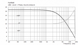
Just a quick sanity check for the phases calculated in ABEC/VACS -
It is for a 1" pulsating sphere in a free field (3D model).
1) The "Farfield=true" option (obviously over-compensated here, as the phase bends up):

2) Explicit "Distance=1m":

3) The above 1m data additionally corrected in VACS for the propagation delay:

This all looks pretty sane to me. It also shows that the phase-wrapped data are perfectly correct, however it may look messy.
BTW, there are actually five curves in each plot (0, 45, 90, 135, 180deg), all being exactly on top of each other - that's also a good check that everything works as expected.
It is for a 1" pulsating sphere in a free field (3D model).
1) The "Farfield=true" option (obviously over-compensated here, as the phase bends up):
2) Explicit "Distance=1m":
3) The above 1m data additionally corrected in VACS for the propagation delay:
This all looks pretty sane to me. It also shows that the phase-wrapped data are perfectly correct, however it may look messy.
BTW, there are actually five curves in each plot (0, 45, 90, 135, 180deg), all being exactly on top of each other - that's also a good check that everything works as expected.
Attachments
Last edited:
I have not found the time to create the LE models for the Tymphany drivers yet.
After Ro808 left his impression that at 800 Hertz, smaller CDs might sound more strained than at 900, I also tried some higher crossover points. 1000 was even a bit better, with a (purely hypothetical) 7.28 Olive score the best result yet on this wavguide, I think due to better transition between both drivers.
1000:


800:


So this is maybe interesting for others working on their waveguide in ath at the moment. I might try to add some more energy below crossover point next. Why? Essentially, it is the interplay between pattern widening around crossover point and cancellation in the interference zone (the nulls) which determinates how smooth the power response falls. So I was thinking, if I added just the right amount of energy, i. e. through a slightly wider pattern for the vertical axis low end, this could even get better. But I have to see if this is possible.
After Ro808 left his impression that at 800 Hertz, smaller CDs might sound more strained than at 900, I also tried some higher crossover points. 1000 was even a bit better, with a (purely hypothetical) 7.28 Olive score the best result yet on this wavguide, I think due to better transition between both drivers.
1000:
800:
So this is maybe interesting for others working on their waveguide in ath at the moment. I might try to add some more energy below crossover point next. Why? Essentially, it is the interplay between pattern widening around crossover point and cancellation in the interference zone (the nulls) which determinates how smooth the power response falls. So I was thinking, if I added just the right amount of energy, i. e. through a slightly wider pattern for the vertical axis low end, this could even get better. But I have to see if this is possible.
^Try adjusting the rotation axis in ABEC/VACS as well, if I understood correctly the rotation axis is through the source by default and this yields error in VituixCAD which assumes rotation axis at mouth. Depending on your waveguide depth this might be significant error and worth checking out if you are going this far with the sims.
You could play with c-c spacing to smoothen the power as well, increase it to >40cm and see what happens 😉 Important thing is to keep the pattern of the waveguide similar to the woofers and you can crossover anywhere below frequency the woofer response gets too narrow, and of course higher than the compression driver is capable to. Ideal situation in the simulator is capable doing these no problem. You can play a lot with this but it kind of revolves around what you already have with slight variations depending on the slopes, delays, physical spacing you use in the simulator.
ps. turn on vertical early reflections on the Power & DI window to see effect of the c-c spacing adjustment.
Last edited:
I think it's important to not let the VituixCAD re-calculate the phases at all - it can't do it right as it knows nothing about the waveguide. It may not be so easy to properly integrate polar data from different software tools. In the next release Ath will do this all in one go, without a need to touch the data afterwards (or specify any offsets, etc.)Try adjusting the rotation axis in ABEC/VACS as well, if I understood correctly the rotation axis is through the source by default and this yields error in VituixCAD which assumes rotation axis at mouth.
Last edited:

- Home
- Loudspeakers
- Multi-Way
- Acoustic Horn Design – The Easy Way (Ath4)