Thanks a lot for your comments, David.
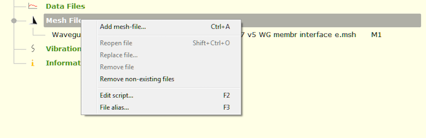
The image showing import of mesh in ABEC got lost somehow during writing. Here it is:
BW,
Christoph
The image showing import of mesh in ABEC got lost somehow during writing. Here it is:
This is a typo. I used Gmsh here exclusively.I see references to Gmsh and also Gmesh.
Gmsh seems popular, do you really use Gmesh too or is it a typo?
BW,
Christoph
Attachments
4. Observation Script: Simulation results using VACS
Thanks Brandon! This is just to support your great work on waveguides presented here a bit from my side...
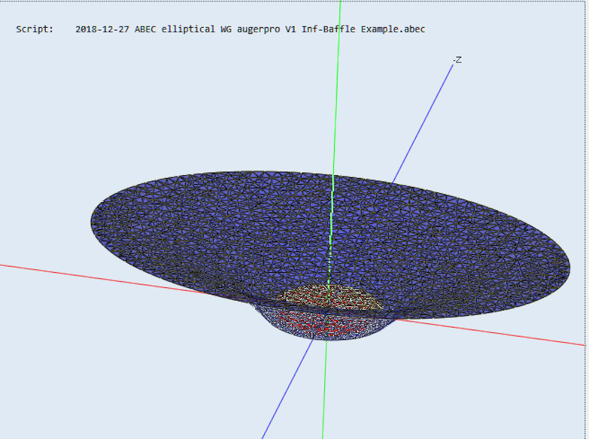
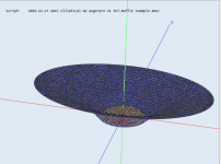
Whatsoever, last step is how to display the simulation results. Before I start over, I wanted to add how the simulated waveguide look like when symmetry is applied:
Back to the observation script: Basically results can be shown as a 'field' directly in ABEC or as 'observation spectrum' using VACS (Visualizing Acoustics Software).
I show how to set up an observation spectrum script to show results via VACS. Again the observation spectrum script is a txt-file, which has to be uploaded to the ABEC project, like the mesh-file earlier. This is just an example, there are more ways to do this (pls refer to the ABEC help). What's in there?
- Nodes
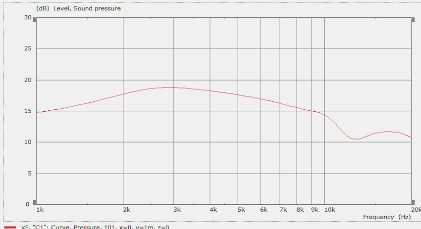
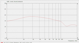
Now that we defined the nodes, we tell ABEC to display an SPL curve in 1000mm distance on 👍-axis as an example:
In VACS this will look like this later (after you let ABEC calculate the spectra):
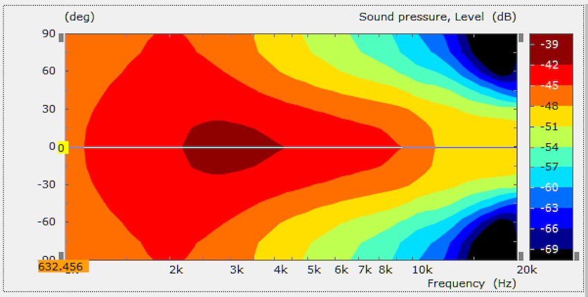
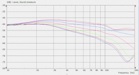
As a second example, we define to depict the horizontal directivity:
How does this look like in VACS?
Please note that you have to do some adjustments in VACS (e.g. frequency range etc) to get exactly this image. Would be an extra post to describe this in detail.
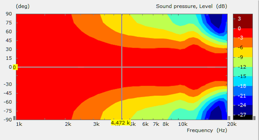
Just as a hint: You can extract quite some additional diagrams/forms of presentation from the data, e.g. the directivity plot can be normalized:
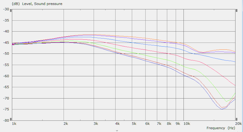
...or single curves under different angles can be depicted (here 0° to +90° in 15°-steps):
Finally, very important: Remember that 'Driving' of the tweeter diaphragm ("HT Front") has been defined in the Boundary Element Script above. Now the 'driving type' and 'Value' has to be defined as 'Driving_Values' in order to get the tweeter diaphragm 'driven' or accelerated:
Please note, that (i) this is just one way to do simulations with ABEC as an example and (ii) this is just a relatively simple start. You could add TSPs of the driver, simulate in a defined enclosure instead of the infinite baffle and so on...
That's it. Very briefly 😉 Hope this helps anyway.
Thanks Brandon! This is just to support your great work on waveguides presented here a bit from my side...
Whatsoever, last step is how to display the simulation results. Before I start over, I wanted to add how the simulated waveguide look like when symmetry is applied:
Back to the observation script: Basically results can be shown as a 'field' directly in ABEC or as 'observation spectrum' using VACS (Visualizing Acoustics Software).
I show how to set up an observation spectrum script to show results via VACS. Again the observation spectrum script is a txt-file, which has to be uploaded to the ABEC project, like the mesh-file earlier. This is just an example, there are more ways to do this (pls refer to the ABEC help). What's in there?
- Nodes
'Nodes' are points in the space defined by a node number and x,y,z-numbers. We need them to define places where e.g. the virtual 'microphone' is placed (here in y-direction, 10, 500 or 1000mm on the y-axis), or on which plane directivity is read out. Again, the scale has to be given and the nodes are defined. Please note, that you can add comments to the script following '//' without messing with scipt commands. Very useful to explain a script or just add notes.Nodes "Spectrum"
Scale=1mm
// Node, x, y, z
1000 0 1000 0 // On-axis 1 m
1001 0 500 0 // On-axis 50 cm
1002 0 10 0 // On-axis 1 cm
2001 0 200 0 //Rotating Point
2002 0 250 0 //Axis direction
2003 100 200 0 //Base plane
Now that we defined the nodes, we tell ABEC to display an SPL curve in 1000mm distance on 👍-axis as an example:
Note that the line '101' refers to node '1000' defined above in nodes 'Spectrum'.BE_Spectrum
PlotType=Curves
RefNodes="Spectrum"
GraphHeader="SPL Box 1m"
BodeType=LeveldB
Range=50dB
101 1000 ID=101 // On-axis
In VACS this will look like this later (after you let ABEC calculate the spectra):
As a second example, we define to depict the horizontal directivity:
Very briefly: With polar range angles (-90° to +90°) and number of simulated angles within this range (13) are defined. The base plane has been defined in Nodes 'Spectrum', other definitions are probably self-explanatory - or explained in the help file.BE_Spectrum
PlotType=Polar
GraphHeader="Polar horiz 1m"
BodeType=LeveldB
Range=30dB
PolarRange=-90, 90, 13
BasePlane=2001 2002 2003 RefNodes="Spectrum"
Distance=1000
101 Inclination=0.0 ID=2101
How does this look like in VACS?
Please note that you have to do some adjustments in VACS (e.g. frequency range etc) to get exactly this image. Would be an extra post to describe this in detail.
Just as a hint: You can extract quite some additional diagrams/forms of presentation from the data, e.g. the directivity plot can be normalized:
...or single curves under different angles can be depicted (here 0° to +90° in 15°-steps):
Finally, very important: Remember that 'Driving' of the tweeter diaphragm ("HT Front") has been defined in the Boundary Element Script above. Now the 'driving type' and 'Value' has to be defined as 'Driving_Values' in order to get the tweeter diaphragm 'driven' or accelerated:
Driving_Values
DrvType=Acceleration
Value=1.0
101 DrvGroup=2001 Weight=1.0
Please note, that (i) this is just one way to do simulations with ABEC as an example and (ii) this is just a relatively simple start. You could add TSPs of the driver, simulate in a defined enclosure instead of the infinite baffle and so on...
That's it. Very briefly 😉 Hope this helps anyway.
Attachments
-
 2018-12-28 ABEC Waveguide symmetry infinite baffle.png421.8 KB · Views: 528
 -
 2018-12-28 ABEC waveguide VACS SPL.png76.4 KB · Views: 529
 -
 2018-12-28 ABEC waveguide VACS hor directivity.png158 KB · Views: 504
 -
 2018-12-28 ABEC waveguide VACS hor directivity norm.png129.6 KB · Views: 508
 -
 2018-12-28 ABEC waveguide VACS SPL 0-90deg.png127.4 KB · Views: 725
@Gaga - wonderful tutorial, many thanks. I hope ABEC can attract a critical mass of supporters and this helps alot.
I noticed you drive the membrane with constant accel, is this a reasonable shortcut? The other alternative (that I see in the Demos) is to use the DrvGroup and RadImp as specified in an LeScript.
Can you point me to a ref that explains how to build the compression driver model? Shortcuts are always welcome.
Hi DonVK,
Thanks a lot.
I used acceleration here in order to keep things simple - and focus on the waveguide contour only. Next step - when you are fine with the WG-contour - would be to simulate a specific driver (did the majority of WG-simulations for the SB26ADC) and use a LE-Script as you describe it. And use the exact membrane geometry of the respective tweeter as well - diameter, height of dome, suspension diameter etc.
Advantage of doing it in two steps is that you learn the impact of the waveguide and the specific driver on the resulting SPL and directivity of the driver-waveguide/horn combination.
Best compression driver model I'm aware of is part of the ABEC example project 'Horn Expo 400'.
Have a look at the limped element script in this project. It describes how the compression driver is set up including a lot of notes and explanations.
The basic principle is to define an electro dynamical driver including its diaphragm:
Then the rear enclosure is described:
A compression chamber in front of the diaphragm is defined (between diaphragm and phase plug):
The phaseplug is simplified and given as a conical waveguide:
In the example, the first part of the horn is modeled again as a waveguide within the LE-script:
I think this model may be a good starting point for own simulations. As said above, I'd start with the simple model, i.e. use a plain disc with the dia of the compression driver exit and acceleration first and intriduce the LE-script based compression driver model later.
An interesting piece of information might be the exit angle of the compression driver and it's coupling to the horn mouth (opening angle).
Thanks a lot.
I used acceleration here in order to keep things simple - and focus on the waveguide contour only. Next step - when you are fine with the WG-contour - would be to simulate a specific driver (did the majority of WG-simulations for the SB26ADC) and use a LE-Script as you describe it. And use the exact membrane geometry of the respective tweeter as well - diameter, height of dome, suspension diameter etc.
Advantage of doing it in two steps is that you learn the impact of the waveguide and the specific driver on the resulting SPL and directivity of the driver-waveguide/horn combination.
Best compression driver model I'm aware of is part of the ABEC example project 'Horn Expo 400'.
Have a look at the limped element script in this project. It describes how the compression driver is set up including a lot of notes and explanations.
The basic principle is to define an electro dynamical driver including its diaphragm:
Def_Driver 'Drv1'
dD=44mm // Diameter of diaphragm
Mms=0.5g // Mass of vibrating assembly
Cms=10e-6m/N // Compliance of suspensions
Rms=4Ns/m // Mech resistances
Bl=5Tm // Motor force factor
Re=6.7ohm // Electrical DC resistance of VC
fre=50kHz ExpoRe=1 // HF modifier of real-part of VC-impedance
Le=0.1mH ExpoLe=0.618 // HF modifier of imag-part of VC-impedance
Then the rear enclosure is described:
Enclosure 'Eb' Node=20
Vb=120cm3 // Effective size of volume
Qb/fo=0.1 // Loss factor
A compression chamber in front of the diaphragm is defined (between diaphragm and phase plug):
Enclosure 'Ef' Node=10
Vb={ dD=44e-3; H=0.5e-3; SD=pi*sqr(dD/2); Vb=SD*H }
The phaseplug is simplified and given as a conical waveguide:
Waveguide 'W1' Node=10=300
STh=3cm2 dMo=1in Len=22mm Conical
In the example, the first part of the horn is modeled again as a waveguide within the LE-script:
The 2in mouth is then coupled to the horn.Waveguide 'W2' Node=300=400
dTh=1in dMo=2in Len=76.5mm Conical
I think this model may be a good starting point for own simulations. As said above, I'd start with the simple model, i.e. use a plain disc with the dia of the compression driver exit and acceleration first and intriduce the LE-script based compression driver model later.
An interesting piece of information might be the exit angle of the compression driver and it's coupling to the horn mouth (opening angle).
^ OK thanks again.
That makes sense to get the WG working then add it to the rest of the model.
I actually did modify the 'expo 400 driver as best I could but some of the parameters were a guess. I'm still looking for a way to extract parameters from a test / measurement because the manufacturers don't provide them.
That makes sense to get the WG working then add it to the rest of the model.
I actually did modify the 'expo 400 driver as best I could but some of the parameters were a guess. I'm still looking for a way to extract parameters from a test / measurement because the manufacturers don't provide them.
Gmsh V4.0
An addition to @Gaga's tutorial on creating meshes for ABEC.
In Gmsh V2 and V3 the [File]->[Save] saves in mesh file format v2.2 which ABEC V3.5 will read properly. The file format version is the first 2 lines of the mesh file.
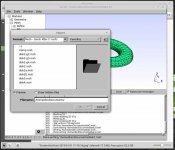
The latest Gmsh V4 saves in file format v4 which is not recognized by ABEC. The newer v4 format contains new tags and elements. If you import there is no object shown and no errors indicated.
However there is a way to export file format 2.2. You need to select [File]->[Export]->[filename : save as]->[format : ascii 2.2]. You don't get to see the file format options until the last step. Some screen shots below.
An addition to @Gaga's tutorial on creating meshes for ABEC.
In Gmsh V2 and V3 the [File]->[Save] saves in mesh file format v2.2 which ABEC V3.5 will read properly. The file format version is the first 2 lines of the mesh file.
Code:
$MeshFormat
2.2 0 8
$EndMeshFormat
The latest Gmsh V4 saves in file format v4 which is not recognized by ABEC. The newer v4 format contains new tags and elements. If you import there is no object shown and no errors indicated.
Code:
$MeshFormat
4 0 8
$EndMeshFormat
However there is a way to export file format 2.2. You need to select [File]->[Export]->[filename : save as]->[format : ascii 2.2]. You don't get to see the file format options until the last step. Some screen shots below.
Attachments

Last edited:
I actually did modify the 'expo 400 driver as best I could but some of the parameters were a guess. I'm still looking for a way to extract parameters from a test / measurement because the manufacturers don't provide them.
Yes, that's true unfortunately. It's difficult to get access to CD TSPs.

Whatsoever, last step is how to display the simulation results..
Thanks once more, and another question.
Patrick posted this is another thread
I asked him about the "jaggies" in the colored plane plots, they look like an artifact of some kind because they are not consistent with the mesh of the horn.
He has not responded, so my question is if you have seen such behavior?
Is this a mesh problem or a VACS/display issue?
Best wishes
David
Also thanks to DonVK for the alert about Gmsh version issues.
Helpful to learn this because I am still at the "how to mesh" step.
Last edited:
I asked him about the "jaggies" in the colored plane plots, they look like an artifact of some kind because they are not consistent with the mesh of the horn.
He has not responded, so my question is if you have seen such behavior?
Is this a mesh problem or a VACS/display issue?
Hi all,
those jaggies/steps or missing field areas do come from mesh and calaculation issues. The solver is trying to solve the pressure/phase whatever in all the triangles in the mesh. When a triangle is touching or even going through the waveguide/wall then we come to this issue: The solver can't solve it, because there is no valid solution for pressure/phase whatever in the wall/waveguide thus it can't display anything and those areas are left empty. Due to rounding errors this might even happen if the mesh is only close but not really touching the wall.
By the way, this issue also leads to long calculation time for the fields.
The solution is paying more attention to the field area/mesh. The mesh should not touch walls or different entities and should left some space between the field and the walls/waveguide.
An easier but not so good solution would be just to increase the mesh resolution, then the steps become smaller - but this will lead to even longer calculation time.
Best Regards
Andreas
those jaggies/steps...do come from mesh... issues.
Hi Andreas
They looked like a mesh problem to me, thank you for the confirmation.
I haven't learned Gmsh yet so it's not clear to me how this occurs, I would expect the mesh code to take care of it but apparently it's an area to watch out for.
I looked at your website, do you use ABEC professionally or another BEM code?
Your expertise in horn optimization leads me to expect you are familiar with Rick Morgans' thesis and publications on the subject from ~2005.
He discusses "source superposition" BEM and I wondered if it had ever become commercialized?
Best wishes
David
Last edited:
Hi David,
you are welcome!
It is no matter of GMSH itself. It doesn't matter where the mesh did come from. The thing is: they should not collide. "They" because there are two meshes here: One for the 3D geometry the system is solved for. And another mesh for the fields, where we want to plot something.
Yes, I do know Richard Morgans thesis as I read it years ago. As I was interested in his optimization method. Quite a good source of knowledge. I know some companies which use their own Matlab code for BEM, maybe they also make use of the super position principle, but as far as I know there is no commercial available solution.
And yes, I am using ABEC professionally. I am also familiar with Comsol Multiphysics, but for my small company it doesn't make sense to invest in it (at least for now), as it is quite expensive. And ABEC is quite powerful for loudspeaker simulations.
Best Regards
Andreas
ABEC test case : memory vs elements vs solve time
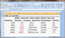
I was curious about the relationship between the model's #elements and the memory and time required to solve it. The solutions are 3D, so as the #elements increases, the time and memory should increase at a cubic rate.
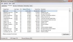
I used a shell model and increased the mesh frequency to force an increase in the #elements. I think the #elements is a good indicator for whether you should go any further, waiting for a potentially long solve time, or pick a new strategy. I used Windows "Task Manager" to check the memory usage over time, and the ABEC reports for the #elements and solve times.
The model is for a 25cm horn, it's compression driver, LR4 XO, and the enclosure. It was just an easy extraction from another project. Its running on a i7-2700K@3.5Ghz with 16GB RAM.
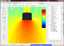
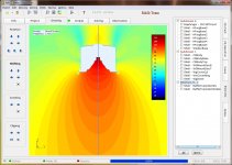
The first 2 pics are the observation fields with and without enclosure+horn+driver shown. The next table has the test results and the last pic is Task Manager. I aborted when ABEC was up to 40GB+ requested, and I have 16GB physical, so the rest was virtual mem (ie. my SSD). It is possible to use up all virtual memory then ABEC will abort with "Out of Memory" error. I don't think I could wait that long for it to solve, so I'll probably keep under 4000 elements.
I was curious about the relationship between the model's #elements and the memory and time required to solve it. The solutions are 3D, so as the #elements increases, the time and memory should increase at a cubic rate.
I used a shell model and increased the mesh frequency to force an increase in the #elements. I think the #elements is a good indicator for whether you should go any further, waiting for a potentially long solve time, or pick a new strategy. I used Windows "Task Manager" to check the memory usage over time, and the ABEC reports for the #elements and solve times.
The model is for a 25cm horn, it's compression driver, LR4 XO, and the enclosure. It was just an easy extraction from another project. Its running on a i7-2700K@3.5Ghz with 16GB RAM.
The first 2 pics are the observation fields with and without enclosure+horn+driver shown. The next table has the test results and the last pic is Task Manager. I aborted when ABEC was up to 40GB+ requested, and I have 16GB physical, so the rest was virtual mem (ie. my SSD). It is possible to use up all virtual memory then ABEC will abort with "Out of Memory" error. I don't think I could wait that long for it to solve, so I'll probably keep under 4000 elements.
Attachments
I was curious about the relationship between the model's #elements and the memory and time required to solve it. The solutions are 3D, so as the #elements increases, the time and memory should increase at a cubic rate.
I used a shell model and increased the mesh frequency to force an increase in the #elements. I think the #elements is a good indicator for whether you should go any further, waiting for a potentially long solve time, or pick a new strategy. I used Windows "Task Manager" to check the memory usage over time, and the ABEC reports for the #elements and solve times.
The model is for a 25cm horn, it's compression driver, LR4 XO, and the enclosure. It was just an easy extraction from another project. Its running on a i7-2700K@3.5Ghz with 16GB RAM.
The first 2 pics are the observation fields with and without enclosure+horn+driver shown. The next table has the test results and the last pic is Task Manager. I aborted when ABEC was up to 40GB+ requested, and I have 16GB physical, so the rest was virtual mem (ie. my SSD). It is possible to use up all virtual memory then ABEC will abort with "Out of Memory" error. I don't think I could wait that long for it to solve, so I'll probably keep under 4000 elements.
Very cool!
Because memory is so darn expensive lately, I was toying with the idea of installing one of those M2 drives to see if that could be (somewhat) competitive with actual RAM.
My laptop, like most, has an M2 slot that's just sitting there empty. So the idea would be to have two tiers of SSD in the laptop, put the operating system and "Program Files" on the Optane, and everything else on an SSD. In Benchmarks, the Optane is well over twice as fast as "top tier" SSDs:
Intel SSD 660p Series Review | StorageReview.com - Storage Reviews
Price is around $100:
Amazon.com: Intel Optane SSD 800P Series (58GB, M.2 80mm PCIe 3.0, 3D XPoint): Computers & Accessories
It's not a huge drive by any means, but my laptop maxes out at 32gb of RAM.
I came close to buying a new desktop this week, but laptops are so darn good these days, it's hard to justify. My laptop sold for $800 and a comparable desktop is only $200 cheaper and about 15% faster.
Sadly, my sixteen core XEON rig bit the dust this week 🙁
Also, I ran some benchmarks this week which were less than scientific, but here goes:
My laptop is a Ryzen 2500U with 16gb of ram. The core clock is 2ghz. One "neat" thing about the Ryzens is that they're so darn efficient, they can 'burst' up to 3.6ghz and they'll throttle back down if things get too hot. When I first started doing ABEC I had an Intel Core i5 laptop and about a third of the time it would get too hot and just crash doing sims. Real fun when a sim has been running for four hours. My Ryzen doesn't have this issue, the laptop doesn't even get particularly hot. Admittedly, older HP laptops had real thermal issues. (I should know, I used to work there and most of us dreaded the older laptops.)
I ran a sim on the Ryzen with forty frequencies from 1000 to 20khz and it took four hours.
I re-ran the same sim on my home theater PC, with 16 frequencies from 1khz to 16khz and it took four hours. My HTPC is an AMD A8 7400K, with four cores running from 3.1 to 3.8ghz.
So, clearly, the Ryzen stomps the A8. This should be no surprise. But the good news is that ABEC seems to run fine on older hardware, as long as you have a decent amount of RAM. My HTPC has sixteen gigs. Which is overkill for a HTPC, but I put it together back when ram was cheap.
they should not collide. "They" because there are two meshes here: One for the 3D geometry the system is solved for. And another mesh for the fields, where we want to plot...
OK, this is the key - I expected that there would be inherent "collision avoidance".
I expected it to be like a "copper pour" on a PCB, where the boundary outline is filled in automatically.
Now I understand.
...I know some companies which use their own Matlab code for BEM, maybe they also make use of the super position principle, but as far as I know there is no commercial available solution...
I couldn't find any either but I wondered if this was just because I wasn't in the industry and my unfamiliarity with what is available.
I am surprised not to find such software because one of Rick's conclusions is that it works faster for comparable accuracy.
Seems to avoid complications such as CHIEF points too.
What do you use with ABEC, Gmsh?
And for the CAD?
To avoid wasted time I want to learn what software works harmoniously, several people in this thread have already identified poorly compatible products.
Very interested in the experience of someone who uses ABEC professionally.
Best wishes
David
I was curious about the relationship between the model's #elements and the memory and time required to solve it. The solutions are 3D, so as the #elements increases, the time and memory should increase at a cubic rate...
More excellent data, thanks once more.
Was this with symmetry exploited?
Symmetry obviously reduces run time but not sure if you would use it for a test case.
Best wishes
David
Very cool!
Because memory is so darn expensive lately, I was toying with the idea of installing one of those M2 drives to see if that could be (somewhat) competitive with actual RAM.
My laptop, like most, has an M2 slot that's just sitting there empty. So the idea would be to have two tiers of SSD in the laptop, put the operating system and "Program Files" on the Optane, and everything else on an SSD. In Benchmarks, the Optane is well over twice as fast as "top tier" SSDs:
Even if you had enough RAM, as soon as the model get a large #elements the solver time is too long to be practical (for me). I'm not even sure if the solver could be partitioned to use GPU(s) which would be ideal.
Also, I ran some benchmarks this week which were less than scientific, but here goes:
My laptop is a Ryzen 2500U with 16gb of ram. The core clock is 2ghz. One "neat" thing about the Ryzens is that they're so darn efficient, they can 'burst' up to 3.6ghz and they'll throttle back down if things get too hot. When I first started doing ABEC I had an Intel Core i5 laptop and about a third of the time it would get too hot and just crash doing sims. Real fun when a sim has been running for four hours. My Ryzen doesn't have this issue, the laptop doesn't even get particularly hot. Admittedly, older HP laptops had real thermal issues. (I should know, I used to work there and most of us dreaded the older laptops.)
Heat is always a problem, especially for laptops. At least you can change the heatsinks and cooling fans in a desktop. I can run my PC 24/7 at 100% load and the CPU never exceeds ambient+20C. If you're thinking of a replacement desktop its helpful to use the online "CPUbenchmark" to compare thread speeds and overall performance. I think the best bang for the buck are those used 2 CPU workstations that typically carry 32-64GB RAM.
Last edited:
OK, this is the key - I expected that there would be inherent "collision avoidance".
I expected it to be like a "copper pour" on a PCB, where the boundary outline is filled in automatically.
Now I understand.
It would be very unfortunate if there is a penalty for observing both inside and outside the speaker because of overlap. I've made no effort to avoid this "interference" or align them. I'll post a few test results as I'm curious to see what effect this has. I never even considered it before.
More excellent data, thanks once more.
Was this with symmetry exploited?
Symmetry obviously reduces run time but not sure if you would use it for a test case.
Best wishes
David
The model I used has 1/4 symmetry, however there are many ways to get to the #element in a model. However you construct the model it should still reduce to a #elements before solving. Another test case 🙂
- Status
- Not open for further replies.
- Home
- Loudspeakers
- Multi-Way
- ABEC experts - help!