I can not follow where that comes from.Vy / Vx = ( 1 - Bnom / ß )
Ok, you said: Bs = Vy = (Vo - Vi) * (-1) = Vi - Vo
Vo = Bn * Vi / Bs
Vi = Vc We look at Bs, that is sampled/sensed beta and is the same for all transistors, so Vi is a constant voltage = Vc
Vy = Vc - Bn * Vc / Bs
Vy = (1 - Bn / Bs) * Vc equal to your equation: Vy / Vx = ( 1 - Bnom / ß )
Your paper example calculations for beta 80, 100, 125 left out Vc.
Your beta curve is normalized (or something) to Bn. Bs becomes zero.
But Vy is not beta! Vy only depends on beta somehow.
So your beta curve follows beta but the actual numeric beta Bs is unknown because Vc becomes Vi which rides on the triangle, and also Bn is unknown.
IMHO from Vy = (Vo - Vi) * (-1) you can visualize the curve but not calculate actual numeric beta.
I did not know what it was, so I guessed "something like 1/beta", but it is normalized.Vbeta-compensation is not beta but something like 1/beta.
Inverting Vbeta-compensation mirrors the curve visually only.
Last edited:
It is not fruitful to start a closed loop equation with this statement: the output of the opamp (U3D) contains the correction (what is sought after), because there is no openloop gain. -> Vout = Ao * [ Vin+ - Vin-]. Sure U3D wants to minimize the error, it differs Ao / [Ao + 1] , which is almost 1, but not exactly.Vi = opamp Vin- = opamp Vin+
Your Vout is my Vz -> Vz = Ao * (Vg - Vx) .
There is a distiction between Vin+ and Vin- (my Vgenerator and Vx-output). Without the openloop gain Ao, it is flattened to equal (and no correction part anymore).Vi = Ic * R * gain...
-> Vx = Aina * Rmeas * Ic .
The gain of the controlled current source is 1, the devider in front is 1/100 ("k4"), R55 specifies the CS-current and is 100ohm (in the eq's 'R5').... & Vo = Ib * R * gain
-> Vz = Ao * ( Vg - (k4 * ß * (Rmeas/R5) * Aina) * Vz (this the closed loop equation, yields to...)
-> Vz / Vg = ( 1/Ao + k4 * ß * (Rm/R5) * Aina ) , the 1/Ao part nullifies.
Now one could extract ß out of this, but this is not usefull: the terms Vg and Vz (opamp output) are still in the eq.
We want the opamp output Vz, containing the original Vgenerator and the correction added to it.
Here kicks in various restrictions and revelations:
Know the expected ß (say: 100x). The Vg is 1V~ but to large for the BJT and the CS, so a devider first (k4), 1/100 (=1/ß).
The CS makes 10mV/100ohm = 100uA base current, the BJT multiplies with ß ('100') to 10mA.
This Ic multiplied with Rmeas (1.00 ohm) is 10mV (again!), the INA multiplies this 100x, Vx output is 1V~ (Vx = almost Vg)
Needed now is the development of the eq towards a Vx - Vz eq.
k4 * Aina = 1 ( 1/ß*ß=1 !!!), R5/Rm = 100 (the expected ß !!!)
Let we take R5/Rm to be the nominal (ideal) ß, naming it 'Bn' (this 'Bnominal' is constant).
-> ß * Vz = (R5/Rm) * Vg (the rest is unity)
-> Vz = (Bn / ß) *Vg
Both sides minus Vg (to remove the Vg part), but we use the Vx because Vx = Vg (!!!).
Vz - Vx = ( (Bn/ß)-1) * Vx
Then the inverter.
Vx - Vz = (1 - (Bn/ß)) * Vx = Vy output (!!!!!)
Vy related to Vx, and not to Vz anymore...
Vy / Vx = ( 1 - Bn/ß ) (Vy = funtion (Vx) )
The X-Y scope or X-Y plotter can show this (#79 picture).
If the datasheet beta is to way off from the above values (k4, Ai, R5/Rm), those need adaptations to suit the actual beta involved.
This is of course an elaborate hardware development, let alone to adapt the circuit to PNP BJT's too!
It lies in the nature of the opamp to equalize Vi+ and Vi- to the most possible extend. If that is not the case, something is wrong with the circuit.
So I see Vi+ = Vi- as a valid assumption.
So I see Vi+ = Vi- as a valid assumption.
Last edited:
That is the point. And the reason why I propose to compute Ic / Ib, because this is undisputable beta.Now one could extract ß out of this
Summary:Vy / Vx = ( 1 - Bn/ß )
Bn is not defined, it is unknown.
Vx is variable with time, it is unknown.
ß is a denominator in the equation...
The correct equation would be:
Vy = ß
Not:
Vy = ( 1 - Bn/ß ) * Vx
Vi+ ≈ Vi- is valid. It cannot be equal or there is no output at all.So I see Vi+ = Vi- as a valid assumption.
The circuit has to be adapted to an expected beta, hence the introduced Bn.Bn is not defined, it is unknown.
Yes and no. Any signal generator is a timed device. Beta as a function of Ic is wanted, time is irrelevant here. There is no time in the ß = f (Ic) specification.Vx is variable with time, it is unknown.
To extract ß, it is made relative to Bn.ß is a denominator in the equation
That would be a certain static value, not a characteristic where ß is related to Ic.The correct equation would be:
Vy = ß
Ic is represented as a voltage Vx, ß is represented as a relative voltage Vy. The oscilloscope is used in the X-Y mode, not in the X-t & Y-t mode.
It seems to me that you could verify the circuit concept in simulation. Does it, or does it not, produce the correct Beta-Versus-Ice plot? Simply use a (simulated) transistor whose Beta-versus-Ice is known beforehand, then connect this transistor model to your measurement circuit. Measure how much your circuit's answer deviates from the known correct answer. Aha, validation & certification.
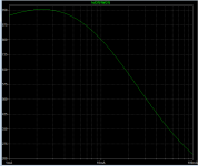
To name one example, the LTSPICE built-in model for the 2N2222 transistor
gives a beta-versus-Ic curve that decreases when Ic increases. LTSPICE simulation plot below.
Incidentally, it's a fun little five minute brain teaser, to discover ways to make LTSPICE create a plot like this. How do you get Ice on the horizontal axis? Woo hoo, plenty of enjoyment.
_
To name one example, the LTSPICE built-in model for the 2N2222 transistor
Code:
.model 2N2222 NPN(IS=1E-14 VAF=100 BF=200 IKF=0.3 XTB=1.5 BR=3
+      CJC=8E-12 CJE=25E-12 TR=100E-9 TF=400E-12 ITF=1 VTF=2
+ XTF=3 RB=10 RC=.3 RE=.2 Vceo=30 Icrating=800m mfg=NXP)Incidentally, it's a fun little five minute brain teaser, to discover ways to make LTSPICE create a plot like this. How do you get Ice on the horizontal axis? Woo hoo, plenty of enjoyment.
_
Attachments
I'm not used with LTspice, and TINA refuses to cooperate with the X-Y scope functionality...
But of course is the proof of the pudding in the eating.
But of course is the proof of the pudding in the eating.
I cenrtainly would like to show it, but this X-Y functionality does not work or I do not know how to. There's no support on the tube alas.Too bad you're unwilling to even try plotting Beta versus Ice in TINA.

"Using_TINA.png" is an image file. The file extension .png signifies that it is of type Portable Network Graphics ... here is Wikipedia's explanation of the details of PNG files, their organization and compression.
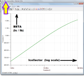
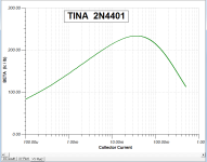
This particular image named "Using_TINA.png" happens to be a screen capture of my laptop, when running Texas Instruments' free circuit simulator TINA. It is a plot of a (TINA simulated) NPN transistor's Beta (Ic/Ib), versus collector current (Ic). The image demonstrates that it is, in fact, possible to make the TINA program plot log(Icollector) on the horizontal axis, and (Ic/Ib) on the vertical axis. All that the circuit designer has to supply, is a little ingenuity. Solve a little brain teaser. Figure out how to get it done, rather than merely Googling "How do I get it done?", then whimpering and muttering when you can't find the answer by trivial searches.
This particular image named "Using_TINA.png" happens to be a screen capture of my laptop, when running Texas Instruments' free circuit simulator TINA. It is a plot of a (TINA simulated) NPN transistor's Beta (Ic/Ib), versus collector current (Ic). The image demonstrates that it is, in fact, possible to make the TINA program plot log(Icollector) on the horizontal axis, and (Ic/Ib) on the vertical axis. All that the circuit designer has to supply, is a little ingenuity. Solve a little brain teaser. Figure out how to get it done, rather than merely Googling "How do I get it done?", then whimpering and muttering when you can't find the answer by trivial searches.
yes, I know what a png is,
Is that refering to one of the here posted circuits ?
Or only about the simulation of a beta curve in general ?
What transistor has beta 1.2k at 100 mA ?
Is that refering to one of the here posted circuits ?
Or only about the simulation of a beta curve in general ?
What transistor has beta 1.2k at 100 mA ?
Spend some hours and shared the effort... ehmm...It is a plot of a (TINA simulated) NPN transistor's Beta (Ic/Ib), versus collector current (Ic). The image demonstrates that it is, in fact, possible to make the TINA program plot log(Icollector) on the horizontal axis, and (Ic/Ib) on the vertical axis. All that the circuit designer has to supply, is a little ingenuity. Solve a little brain teaser.
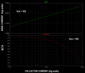
Here's a typical example of the difference between datasheet and circuit simulation (in this case: TINA), using .MODEL parameters.
When you get your tester working and accuracy verified, you can show examples of the difference between datasheet and measurements on actual real-life devices.
_
When you get your tester working and accuracy verified, you can show examples of the difference between datasheet and measurements on actual real-life devices.
_
Attachments
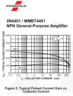
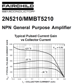
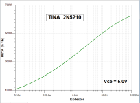
Another example. Again TINA simulation is not a wonderful match to the datasheet.
However, as proposed in post #89 above, you could drop this TINA-simulated 2N5210 transistor into a TINA-simulation of your Beta-versus-Icollector hardware device. As long as your TINA-simulated results from the simulated hardware device, match the raw Beta-versus-Ic from a TINA simulation of the transistor without the hardware device . . . . you know the hardware device got the right answer. It extracted a Beta-versus-Ic curve which approx. matches how the simulator says the raw transistor behaves.
_
Attachments
- Home
- Design & Build
- Equipment & Tools
- Transistor HFE - IC curve tracer?