Hi All,
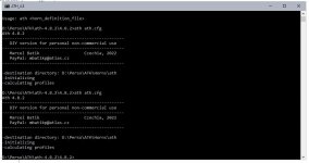
I'm training on ATH and can't get STL output.
May you please check my config file ?
Thanks.
Edit : I only get a mesh.geo file.
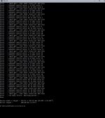
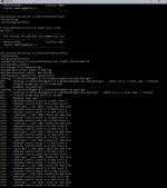
And attached is the return of CMD, no dimensions displayed.
I'm training on ATH and can't get STL output.
May you please check my config file ?
Thanks.
Edit : I only get a mesh.geo file.
And attached is the return of CMD, no dimensions displayed.
Attachments
Last edited:
- The first three lines from your script are for the ath.cfg which is a global config file. Use a different file for a WG project (the rest of your script).
- For some reason STL is not correctly generated when Output.ABECProject=0. Try setting it to 1. I'll check that.
- For axisymmetric devices there's a much better way - see ABEC.SimProfile=0.

Use the latest executable -
https://www.diyaudio.com/community/...-design-the-easy-way-ath4.338806/post-6996527
https://www.diyaudio.com/community/...-design-the-easy-way-ath4.338806/post-6996527
Regarding the delay compensation in general, I forgot to explicitely mention one thing - when you normalize the data (NormAngle=0), the phase is normalized as well (i.e. all is relative to the on-axis response). That's why we have Distance = 2.0 and PhaseComp = -2.0, effectively eliminating any delay compansation in this case, as 2 and -2 cancel out. We don't want any compensation in this case, as the default value would add negative delay (~2m) to what is already "flat". I hope it makes sense.[...] Also, when I enter an offset with the offset parameter, must this be added/subtracted from phase compensation?
Last edited:
Flip the MapAngleRange to 180,-180, 72 and it should go the other way. Starting at plus 180 going round to -180.
I had thought so to, but ABEC does not accept this range and gives the following prompt under observation scripts:
Code:
PolarRange= values missing in "PolarRange"Removing the delay to unwrap phase is what I understood to be the operation here, as in REW. That perfectly makes sense. So, when distance defines the virtual microphone/measuring spot, it comes natural that we'd remove this from the signal. If offset is not adding anything to distance, and source <-> measuring spot is simply shifted for a new rotation center, I understand that no further action is needed.I hope it makes sense.
Can't find how to set a different coverage angle for horizontal and vertical for rectangular horn.
Ex :
140x80mm mouth
100° horizontal
60°vertical
Thanks.
Ex :
140x80mm mouth
100° horizontal
60°vertical
Thanks.
Last edited:
http://www.at-horns.eu/release/Ath-4.8.2-UserGuide.pdf#page=10
- In the meantime I'm working on an option of having two separate - horizontal and vertical - profiles, and creating truly rectangular horns. I'd like to have the possibility to explore some diffraction slot geometries. There are still quite a lot of unknows there for me.
For now, what's described in the documentation are "the only" options.
Last edited:
Manually or through Ath change the Inclination to 180 in the observation script to flip it around.I had thought so to, but ABEC does not accept this range and gives the following prompt under observation scripts:
Code:PolarRange= values missing in "PolarRange"
Code:
BE_Spectrum
  PlotType=Polar; GraphHeader="V Polar Down"
  PolarRange=0,180,37
  Farfield=true; BasePlane=zy
  Distance=2m
  //Offset=200mm
  //NormalizingAngle=10
  502  Inclination=0  ID=5002

BE_Spectrum
  PlotType=Polar; GraphHeader="V Polar Up"
  PolarRange=0,180,37
  Farfield=true; BasePlane=zy
  Distance=2m
  //Offset=200mm
  //NormalizingAngle=10
503 Inclination=180 ID=5003http://www.at-horns.eu/release/Ath-4.8.2-UserGuide.pdf#page=10
- In the meantime I'm working on an option of having two separate - horizontal and vertical - profiles, and creating truly rectangular horns. I'd like to have the possibility to explore some diffraction slot geometries. There are still quite a lot of unknows there for me.
For now, what's described in the documentation are "the only" options.
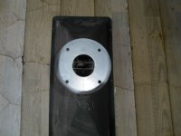
This is great, I wrote my own scripts to make the meshes for these types of horn in OCTAVE/MATLAB as they seem to be the only way to get wide coverage and good low frequency loading but my software is not as sophisticated as ATH4. This EV HP640 is a particularly sophisticated horn that makes used of a exponential-conic-conic expansion and has vanes in the throat to reduce the HF narrowing.
Attachments
Manually or through Ath change the Inclination to 180 in the observation script to flip it around.
I was using -180, 180, 72, and changed it to 180, -180, 72. The first command works for a full spin, but gives reversed orientation, the second leads to the aforementioned complaint from ABEC.
This EV HP640 is a particularly sophisticated horn that ...
You mean: it's a diffraction horn?!
I also wanted to ask @kimmosto, here is another observation of the new ath capabilities:


First DI/ERDI curve is the product of VCad, combination of SPL Trace tool and Diffraction tool for a baffle of 57 cm by 32 cm with 4 cm edge rounding, for the woofer PHL 3411. Second DI/ERDI curve is based on the Sd of PHL 3411, converted into cicular radius and used in ath 4.8.3 beta for BEM simulation in an enclosure of 57 cm by 32 cm by 27 cm (HxWXD), with a 2.5 cm edge rounding. In both cases, positioning of the woofer is about the same. But quite a difference between 1 and 2k (the upper frequencies are of no concern). What to rely on?
First DI/ERDI curve is the product of VCad, combination of SPL Trace tool and Diffraction tool for a baffle of 57 cm by 32 cm with 4 cm edge rounding, for the woofer PHL 3411. Second DI/ERDI curve is based on the Sd of PHL 3411, converted into cicular radius and used in ath 4.8.3 beta for BEM simulation in an enclosure of 57 cm by 32 cm by 27 cm (HxWXD), with a 2.5 cm edge rounding. In both cases, positioning of the woofer is about the same. But quite a difference between 1 and 2k (the upper frequencies are of no concern). What to rely on?
I'm not sure of the exact definition as any horn that isn't an infinite conical horn has diffraction. In this horn all the initial expansion is in the horizontal plane and no initial vertical expansion but also it dosen't 'pinch' down like many horns described as a diffraction horn.You mean: it's a diffraction horn?!
I think starting at 0 makes the most sense and using the zy plane. In my example above the V up goes from on axis to 180 in the upper hemisphere and by flipping the inclination V down goes the other way. This is how I would measure the speaker.I was using -180, 180, 72, and changed it to 180, -180, 72. The first command works for a full spin, but gives reversed orientation, the second leads to the aforementioned complaint from ABEC.
I see hardly any difference that isn't due to the application of the traced on axis response. If you want to compare the difference between Vituix and the Ath generated woofer don't trace the on axis and just use the diffraction tool. If there is any real difference there it will be due to the depth of the cabinet which is not considered by Vituix, and therefore the full 3D simulation is more likely to be accurate in simulating the directivity.But quite a difference between 1 and 2k (the upper frequencies are of no concern). What to rely on?
I was testing this and the result is that differences are probably resulting from the added third dimension, depth. Especially the diffraction waves must be a result of enclosure depth, as well as the slightly lower DI.I see hardly any difference that isn't due to the application of the traced on axis response. If you want to compare the difference between Vituix and the Ath generated woofer don't trace the on axis and just use the diffraction tool. If there is any real difference there it will be due to the depth of the cabinet which is not considered by Vituix, and therefore the full 3D simulation is more likely to be accurate in simulating the directivity.
Hi Mabat, Hi All,
About the coverage angle, may you please explain a bit the way to get 90° horizontal and 60° vertical ?
We currently set en angle :
Coverage.Angle = 45 for 90° overall coverage.
What to add to reduce the angle from 90° to 60° on Z axis ?
Thank you, it's still not clear for me.
This is my current .cfg file :
Throat.Profile = 1 ; 1 = OS-SE waveguide
Throat.Diameter = 13 ; [mm]
Throat.Angle = 5 ; half the included angle [deg]
Coverage.Angle = 45 - 10*cos(20)^2 ; half the included angle [deg]
Length = 70 ; [mm]
Term.s = 1
Term.n = 5.0
Term.q = 0.996
OS.k = 1
Morph.TargetShape = 1 ; 0 = no morphing (the default)
Morph.TargetWidth = 140
Morph.TargetHeight = 80
Morph.CornerRadius = 10
Morph.FixedPart = 0
Morph.Rate = 3
Morph.AllowShrinkage = 1
Mesh.AngularSegments = 120 ;64
Mesh.LengthSegments = 50 ;20
Mesh.ThroatResolution = 2.0 ; 4.0[mm]
Mesh.InterfaceResolution = 4.0 ; 8.0[mm]
Mesh.InterfaceOffset = 2.5 ; 5.0[mm]
Output.STL = 1
Output.ABECProject = 1
Last edited:
You can either use a guiding curve (ellipse or superellipse), or use the following formula for the Coverage.Angle:
Coverage.Angle = 90 - (90-60)*sin(p)^2
See https://www.desmos.com/calculator/mnubszwpe0
Coverage.Angle = 90 - (90-60)*sin(p)^2
See https://www.desmos.com/calculator/mnubszwpe0
Would you have some sim results to share? I would expect these devices to be very resonant. My aim is to explore what can be done about that.I wrote my own scripts to make the meshes for these types of horn in OCTAVE/MATLAB [...]
- Home
- Loudspeakers
- Multi-Way
- Acoustic Horn Design – The Easy Way (Ath4)