...then think i try merge tails from post 511 where the off axis curves is cut.
Great -- thanks for doing all this! I am looking forward to the outcome!
Just to understand the tweeter DI behavior, in the attached plot, I have compared the directivity index of the Scanspeak R2904 with WG148 waveguide mounted in the cabinet of Pida (violet curve) and the Monkey box cabinet (red curve).
The cabinet made by Pida is designed with curved cabinet edges. As far as I can understand it at this moment, that is the reason for the different DI curves.
I don't see it as a problem in the Monkey Box, because we have agreed at the start of the project to keep the cabinet simple.
Yes, we deliberately made the "flat baffle" compromise right at the beginning. The models told us that we can spread out dips/peaks in the SPL response resulting from the baffle-edge diffraction by placing the drivers off-center, which seems to work to prevents any "bad" dips/peaks so far. The waveguide also helps to reduce the baffle-diffraction effects by focusing the sound away from the edges. This already works okay with the WG148, and we might get another option with the augerpro waveguide later on. I must say that I have seen worse dispersion patters, and I guess the dispersion we get with the current setup is, overall, not too bad.
For the next steps I'd suggest the following:
- Take a look at the dispersion analysis with the current x-over draft (try with VituixCAD, or else resort to Leap)
- Tweak the x-over circuit (if necessary)
- Build prototype filter and do measurements
- Compare measurements with modeled data, tweak prototype filter accordingly
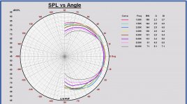
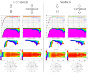
Out of the horizontal off axis 90 to -90 degrees SPL sum of the filtered midrange and tweeter, I created the horizontal polar diagram using a polar convertor from 1 - 10 kHz. Also a version, normalized to the on axis response.
It looks not bad. You can see the SPL asymmetry inside and outside caused by the asymmetric position of the drivers on the front baffle.
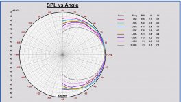
As an info, in the plots the beam bandwidth BW and the directivity index DI are listed also for the different frequencies.
It looks not bad. You can see the SPL asymmetry inside and outside caused by the asymmetric position of the drivers on the front baffle.
As an info, in the plots the beam bandwidth BW and the directivity index DI are listed also for the different frequencies.
Attachments
Last edited:
I think low frequency data to Vituixcad is measured near field (couple of millimeters), woofer and port. Then use diffraction tool to woofer data (baffle). Then choose merge frequency for near and far field response.
Below results is after merge tails for 1 meter off axis response with results seen in the last three REW overlays, also VituixCAD zip folder is attached, unzip that folder to users path Documents\VituixCAD\Projects\Monkey_BOX. A quick navigating hint for first time in VituixCAD is try double click on the six plots to maximize and double click again to minimize, also right click into each of six plots give nice possibilityes, up at top one can change reference angle to minus or plus side of speaker which make nice interesting changes to power response and directivity index curves on the fly.
Attachments
Last edited:
Out of the horizontal off axis 90 to -90 degrees SPL sum of the filtered midrange and tweeter, I created the horizontal polar diagram using a polar convertor from 1 - 10 kHz. Also a version, normalized to the on axis response.
It looks not bad. You can see the SPL asymmetry inside and outside caused by the asymmetric position of the drivers on the front baffle.
Nice! I am not worried about the slight asymmetry, as long as things are nice and smooth without any bad peaks/dips.
I think low frequency data to Vituixcad is measured near field (couple of millimeters), woofer and port. Then use diffraction tool to woofer data (baffle). Then choose merge frequency for near and far field response.
No need for that. I did some anechoic measurements down to 80 Hz or so, and these were used to "tune" the baffle diffraction model in Leap, and to splice the modelled low-frequency model at 1m to the measured dispersion data. See post 511.
Below results is after merge tails for 1 meter off axis response with results seen in the last three REW overlays, also VituixCAD zip folder is attached...
Great! Splicing looks ok to me. I have not yet tried to work with the Vituix data myself. The off-axis charts look mostly okay. The vertical off-axis shows the expected features at the x-over frequencies, but not bad. The sharp cut-off filters seem to pay off.
The horizontal off-axis charts show a few things at the x-over frequencies:
- There is a slight dip a the woofer/mid x-over in the on-axis response, and this dip carries over to the off-axis response. Would it make sense to slightly incease the woofer/mid overlap to reduce this dip?
- The on-axis response is pretty flat at the mid/tweeter x-over, but it shows a peak in the off-axis response. What's the best way to deal with this? Reduce the overlap a bit, compromising the on-axis response?
...Great! Splicing looks ok to me. I have not yet tried to work with the Vituix data myself. The off-axis charts look mostly okay. The vertical off-axis shows the expected features at the x-over frequencies, but not bad. The sharp cut-off filters seem to pay off.
The horizontal off-axis charts show a few things at the x-over frequencies:
- There is a slight dip a the woofer/mid x-over in the on-axis response, and this dip carries over to the off-axis response. Would it make sense to slightly incease the woofer/mid overlap to reduce this dip?
- The on-axis response is pretty flat at the mid/tweeter x-over, but it shows a peak in the off-axis response. What's the best way to deal with this? Reduce the overlap a bit, compromising the on-axis response?
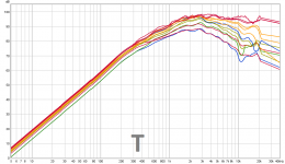
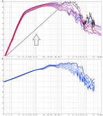
Maybe i didn't merge good enough really don't know and maybe that provocate the power response dip aroud 500Hz, for info spliced all of them around 300Hz point more or less brutal. What i mean is below in a camparison to the demo "Epe-3W_demo.zip" project where we see say below about 700Hz could maybe be better and make a difference. To explain those REW overlay graphs, top plots is monkey box and bottoom plots are from that VituixCAD demo "Epe-3W_demo.zip", colors for monkey box is black for on axis and red are right side and blue is left side at axis 0º/15º/30º/45º/60º/75º/90º, and for demo black is on axis and because its a symetric baffle only left side is plotted at axis 0º/15º/30º/45º/60º/75º/90º. Also saw some talk down the road ablout a 1,5dB difference so will ask is there a chance those off axis curves in general shoul be increased +1,5dB before merged with on axis low end tail.
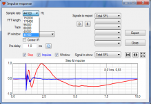
BTW in previous post forgot hang on estimated system IR/SR @96kHz.
Attachments


Last edited:
Maybe i didn't merge good enough really don't know and maybe that provocate the power response dip aroud 500Hz, for info spliced all of them around 300Hz point more or less brutal.
I don't see how the hard splicing at 300 Hz can affect the result at 500 Hz. I guess you might just do the whole analysis with just the anechoic data >300 Hz without splicing.
And then we still have the off-axis peak at 2.5 kHz, which actually looks more important than the 500 Hz dip to me.
BTW in previous post forgot hang on estimated system IR/SR at 96kHz.
Interesting! Can you export that in a data file that allows importing to other software?
Last edited:
I don't see how the hard splicing at 300 Hz can affect the result at 500 Hz. I guess you might just do the whole analysis with just the anechoic data >300 Hz without splicing...
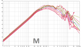
Problem seems in the 12 off axis curves they stop abrupt at 300Hz then software interpolate a tail below and that tail was seen in first run that it boosted too much low shelve energy below that 300Hz point, so think there is no way out of manipulate below 300Hz to something real world realistic. I have a look tonight and see how it looks add +1,5dB and maybe merge a little higher in frq to get them look more like demo from kimmosto.
...And then we still have the off-axis peak at 2.5 kHz, which actually looks more important than the 500 Hz dip to me...
Its possible bypass what ever schematic components and one can even for momentary use throw in some unlimeted power of digital blocks just to see if its possible improve that region, will try later but lets see if its repairable at all because at those frq design spacing/alligment/polars can mean alot and hard to do wonders about.
...Interesting! Can you export that in a data file that allows importing to other software?
It looks like, at what samplerate ?
Attachments
Last edited:
Problem seems in the 12 off axis curves they stop abrupt at 300Hz then software interpolate a tail below and that tail was seen in first run that it boosted too much low shelve energy below that 300Hz point ... get them look more like demo from kimmosto.
I don't think so. The low-frequency part you used came from the Leap model, which was tuned by anechoic measurements (above 80 Hz). The kimmosto example curves look like their low-frequency part was done by extrapolating the anechoic parts of the impulse responses in some way in order to allow longer FFTs, which in turn give rather meaningless low-frequency SPL data (not something I'd recommend to do in this situation).
It looks like, at what samplerate ?
44100 Hz is good. Everything higher does not contain anything meaningful because I made the measurements at 44100.
...44100 Hz is good...
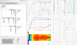
Hanged on below for system plus individual passbands, system IR imported to REW waterfall show below visual when looking 20dB down using the included window settings.
Attachments
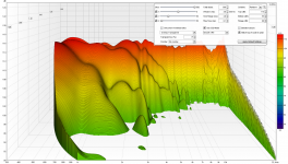
Hanged on below for system plus individual passbands, system IR imported to REW waterfall show below visual when looking 20dB down using the included window settings.
I tried to take a look at those data files. Two questions:
- The impulses start at about 1ms, which corresponds to about 0.3m from the baffle. Are these data really the results for the microphone 1m away from the baffle?
- What is the scaling / physical units of the amplitude values? Pascals? It seems the different data files use different scaling / units.
Last edited:
I tried to take a look at those data files. Two questions:
- The impulses start at about 1ms, which corresponds to about 0.3m from the baffle. Are these data really the results for the microphone 1m away from the baffle?
- What is the scaling / physical units of the amplitude values? Pascals?
Admit had been too lazy to read up on that IR stuff and why it change centering or amplitude from software to software, about amplitude a guess is its sort of normalize process so we can load that IR into a player or convolution engine and get a kind of standard SPL, neigher amplitude or time alignment of IR is a problem into for example REW where one can offset amplitude and allign time to be centered or whatever wishes there can be. If used software can not manipulate with IR as REW can then think its possible use free Audacity to move IR that 1mS in time and also it should be able change level of amplitude. For info number for system sum amlitude allignment at 1kHz is 90,8dB into VituixCAD.
For the next steps I'd suggest the following:
- Take a look at the dispersion analysis with the current x-over draft (try with VituixCAD, or else resort to Leap)
- Tweak the x-over circuit (if necessary)
- Build prototype filter and do measurements
- Compare measurements with modeled data, tweak prototype filter accordingly
Matthias:
- I will do a good review of the xo w.r.t. phase response and also the power response, in order to know if the schematic is optimal. Maybe some little compromise has to be done with the on axis response.
- for the woofer off axis I need to do some Leap off axis simulations and splice them with your measurements. Then I will have a good view on the woofer-midrange sum off axis also. It is possible that the woofer fall off maybe is a little too high off axis, resulting in some SPL dip. I have to look at it.
It can take some time as I have also my own speaker playing tomorrow. But I will do soon.
Byrtt: I look too your results soon, too occupied now. It looks that VituiXCAD is an interesting tool for post processing measured data. Together with a powerful diffraction calculator it can be a replacement maybe for Leap (which is becoming old).
I am slowly getting the hang out of VituixCAD, and I played a bit with the Monkey Coffin "simulation" files in post 544. My impression is that the off-axis dip at the woofer/mid x-over might be an artifact resulting from different measurement setups and data processing of the on-axis (outdoor) and on-axis (indoor) data. The on-axis SPL curve has a nice resolution in the 500 Hz range, because this curve relies on on the outdoor measurements, which have a longer anechoic impulse response and therefore provide higher FFT resolution. The off-axis data have much less frequency resolution, so the narrow x-over range at 500 Hz is not resolved well in these data. Comparing these on-axis and off-axis data in the narrow x-over band at 500 Hz therefore does not seem right, and the dip in the acoustic power (integrated around the speaker) seems to be an artifact from this. To avoid this artifact at the woofer/mid x-over frequency, the on-axis and off-axis SPL curves need to be measured and processed in the same way. This seems like the only way to go if we need to study the directivity at the woofer/mid x-over in order to optimize the filter.
The best solution would be to do a full set of off-axis outdoor measurements at all angles. This would give sufficient frequency resolution to show what's happening at the woofer/mid x-over. However, for practical reasons, this is very difficult, and we'll have to cope with this issue in some other way.
As an alternative, we could use a model tool to estimate the low-frequency part of the SPL curves of the woofer and the mid (!) up to about 700 Hz or so (at all angles!), and splice these to the indoor measurements. I have tried doing this in Vituix, but I did not really understand what Vituix was doing (or Vituix did not understand what I wanted). Maybe Leap would work out for this?
However, I wonder if we really need to do all of this. Why would there be a (serious) issue with directivity at the woofer/mid x-over anyway? I may have missed something, but if there is no good reason for such issues, we could just assume that if the on-axis response is flat (where we have data with good frequency resolution) the off-axis response is also smooth. I guess the issue would be more relevant at the mid/tweeter x-over, where the directivities of the waveguides come into play.
Sorry for this long and complicated post... Let me know what you think.
Last edited:
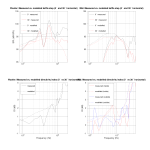
Thinking a bit more about how to model the low-frequency dispersion of the Monkey Coffin I compared the outdoor measurements on-axis and 30° horizontal off-axis (anechoic, frequency resolution better than 90 Hz). I also added the Vituix baffle diffraction model to the comparison. See attached plots.
Top panels: measured SPL on-axis and 30° off axis, together with Vituix baffle diffraction model (left: woofer, right: midrange). Note that the woofer SPL measurements are polluted by the resonances from the bass reflex port (big peaks and dips). Of course, the Vituix diffraction curves do not match the driver SPL curves, but that's not the point.
Bottom panels: difference between the on-axis and off-axis SPL curves (measured and modelled). This is the directivity index.
It seems that Vituix does a reasonably good job to predict the directivity index.
This means we could use the Vituix diffraction calculator to estimate the off axis SPL curves at low frequencies from the on-axis SPL curves of the woofer and the midrange driver (without the x-over). Using the outdoor measurements with about 80 Hz resolution, we could therefore model the off-axis response curves with the same frequency resolution even at low frequencies.
This approach might provide us with more useful dispersion data that would allow optimizing the circuit of the woofer/mid x-over at about 500 Hz, taking into account the on-axis and off-axis SPL curves in a good way.
What do you guys think?
Attachments
@mbrennwa, Paul Vancluysen
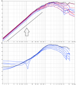
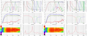
You are the specialist and know when measurement data is in agreement and to trust, in meantime for fun i manipulated on axis curves so when cascaded with electric filter slopes on axis system gets mostly close to Paul's textbook slope targets, see below the small changes where the sixpack plots at left have the textbook slopes on axis but the same seven off axis responses as in the right six pack plots, not much of a change for power response mostly its directivity index that show a difference.
You are the specialist and know when measurement data is in agreement and to trust, in meantime for fun i manipulated on axis curves so when cascaded with electric filter slopes on axis system gets mostly close to Paul's textbook slope targets, see below the small changes where the sixpack plots at left have the textbook slopes on axis but the same seven off axis responses as in the right six pack plots, not much of a change for power response mostly its directivity index that show a difference.
Attachments
...
The combination 2nd order Bessel at 500 Hz and 3rd order elliptical at 2500 Hz (Kaffimann proposal) has IMO the disadvantage that the midrange SPL passband is not flat.
...
I would actually suggest 2nd order Bessel LP for the woofer, 3rd order Butterworth HP for the mid, and elliptic for the mid/tweet. Has to be adjusted accordingly, remember to use the drivers frequency response together with xo points or the effort is wasted.
If you want to use Bessel for woofer/mid it would have to be offset, but IMO all the filters should be slightly offset anyway, regardless of type, order and slopes.
*sigh* I will have to look into Vituix then, have not gotten around to it, even though I am donating a tiny sum regularly. Can I just import the FRD files and it's all good to go?
@mbrennwa, Paul Vancluysen
... in meantime for fun i manipulated on axis curves so when cascaded with electric filter slopes on axis system gets mostly close to Paul's textbook slope targets, see below the small changes where the sixpack plots at left have the textbook slopes on axis but the same seven off axis responses as in the right six pack plots, not much of a change for power response mostly its directivity index that show a difference.
Byrt:
it is not clear for me, what exactly did you change in the right six pack plots w.r.t. to left ones. And which seven off axis repsonses are you talking about, the measured ones by Mattias or some spliced ones. Maybe I have missed something, because I didn't analyse the previous posts in detail, sorry for that.
I would actually suggest 2nd order Bessel LP for the woofer, 3rd order Butterworth HP for the mid, and elliptic for the mid/tweet. Has to be adjusted accordingly, remember to use the drivers frequency response together with xo points or the effort is wasted.
If you want to use Bessel for woofer/mid it would have to be offset, but IMO all the filters should be slightly offset anyway, regardless of type, order and slopes.
*sigh* I will have to look into Vituix then, have not gotten around to it, even though I am donating a tiny sum regularly. Can I just import the FRD files and it's all good to go?
Kaffimann:
Your propsal is to combine a 2nd order Bessel low pass on the woofer with a third order Butterworth high pass on the midrange. I am wondering, what about phase aligning of the filtered drivers and the polar response of the sum, especially in the vertical direction.
Do you have a practical example or article where this combination is used or described in? I can look to it my self also, making some target curves and look to the behavior of the sum response. For me this is new.
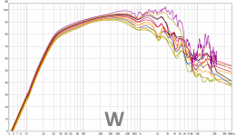
I have done an off axis simulation in Leap to compare with the indoor measurements of Matthias.
There is a large difference between the simulation and the measurements.
In the plot the SPL off axis of the Faital 12PR320 0 - 30 - 60 deg on - off axis. Measurements in color, simulations in black.
I dont't understand it. I have some older off axis measurements of an 11 inch in a cabinet, done in a professional anechoic room. I will have a look at those also.
Remark that ka = 1 at 439 Hz for the used 12 inch woofer.
As an information, this is the transition frequency between non-directional and directional radiation (on infinite baffle).
I will investigate this, we have to be sure which are correct off axis curves if an off axis study of the woofer is wanted...
Attachments

Last edited:
- Home
- Loudspeakers
- Multi-Way
- Open Source Monkey Box