It is well laid out in "Measuring SPL" here: SoundEasy Design Guide This is for Soundeasy, but the principle is exactly the same regardless of software. It's a method that works great, better IMHO than other competing methods when you balance all the pros and cons of each (ungated, smoothed in-room, or variable gating, for example).
Yes I know this site, very good studies to find there.
We will try out this diffraction calculator also
")
I did use Jef Bagby baffle edge diffraction calculator for the Volt midrange in the Monkey Box baffle and compared with the Leap simulation.Little difference but very comparable.
Could you plot the diffraction curves from post 438 along with the difference between my nearfield measurement and the Leap response curve of your post 436? Just from eyeballing the two plots I would not be surprised if all three curves would line up nicely, and it might tell us a bit more about how to go with the splicing.
Guys, remember that the Volt midrange is a dome in a waveguide with straight edges. It's nearfield measurement vs. farfield don't follow rules for planar radiators - simulations fail!
Respose measured in farfield, with the baffle used for the actual speaker is needed, just take care of artefacts that come from floor/wall reflections.
Respose measured in farfield, with the baffle used for the actual speaker is needed, just take care of artefacts that come from floor/wall reflections.
Guys, remember that the Volt midrange is a dome in a waveguide with straight edges. It's nearfield measurement vs. farfield don't follow rules for planar radiators - simulations fail!
I would be surprised if the "horn" does much below 1 kHz, where the wavelengths are quite a bit larger than the horn.
Matthias,
I hope I understood your question well, otherwise tell me.
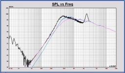
I have calculated the bafflesteps with three SPL curves and the Bagby one:
- nearfield measured (black)
- infinite baffle Leap, model based on measured TSP (no frequency response correction applied at high frequencies) (pink)
- in cabinet Leap, model based on measured TSP (no frequency response correction applied at high frequencies) (blue)
The nearfield response scaled to be equal to the Leap infinite baffle response for low frequencies.
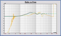
The bafflesteps:
- yellow = transfer SPL Leap in cabinet over SPL nearfield
- black = transfer SPL Leap in cabinet over Leap SPL infinite baffle
- green = Jeff Bagby
I hope I understood your question well, otherwise tell me.
I have calculated the bafflesteps with three SPL curves and the Bagby one:
- nearfield measured (black)
- infinite baffle Leap, model based on measured TSP (no frequency response correction applied at high frequencies) (pink)
- in cabinet Leap, model based on measured TSP (no frequency response correction applied at high frequencies) (blue)
The nearfield response scaled to be equal to the Leap infinite baffle response for low frequencies.
The bafflesteps:
- yellow = transfer SPL Leap in cabinet over SPL nearfield
- black = transfer SPL Leap in cabinet over Leap SPL infinite baffle
- green = Jeff Bagby
Attachments
Last edited:
The bafflesteps:
- yellow = transfer SPL Leap in cabinet over SPL nearfield
- black = transfer SPL Leap in cabinet over Leap SPL infinite baffle
- green = Jeff Bagby
Ok, the yellow curve does not do the same thing as the "theory" curves. Either the theories are incomplete, or the dome/horn does indeed behave differently than conventional cones.
Theory: as far as I can tell, the baffle diffraction calculators assume "perfect" dispersion (spherical sound emission) to estimate how much sound hits the baffle edges. Is this really the case?
Dome/horn: as mentioned before, the nearfield 2.4 kHz peak is interesting, as this is a dip in the far field. I made a quick nearfield test with the microphone off-center (approximately in front of the dome surround), and the peak was almost gone. So yes, funny things do happen in the dome/horn system. Maybe such things also happen at around 400-500 Hz, and are confusing our view on the splicing. However, the wavelengths involved would be quite a bit larger than the horn, so I find it hard to believe that.
Splicing at 1 kHz might be the way to go (as suggested by Paul). However, I am not very experienced with splicing + modeling, so I leave it up to Paul and others to decide on a workable approach. Let me know if there's anything I could do in terms of measurements.
I agree that at lower frequencies the horn *should* be relatively ineffective. So pushing the splice to where the far field measurement cutoff is, is the way to go. You want to preserve the measured far field phase as low as possible.
Also most diffraction sims model driver directionality, of course they typically assume a flat piston though.
Also most diffraction sims model driver directionality, of course they typically assume a flat piston though.
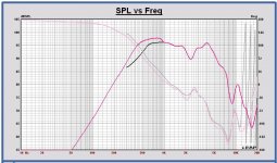
For the midrange I have done a SPL data splice of the Leap simulation and the measured curve.
Following steps:
- applied a minimum phase transform on the measured SPL
- compensated excess delay of measured phase to fit on minimum phase; compared both; minimum phase can be used.
- SPL data splice at 980 Hz
- minimum phase transform on data spliced curve to smooth little phase discontinuity at splice frequency.
In first plot amplitude and phase of data spliced curve (red) and the measurement, excess delay compensated (black)
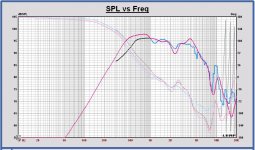
In the second plot with simulated curve added (blue) to see the way of splicing.
I don’t feel so good with the SPL difference of measurement and simulation below 1 kHz. The data spiced curve is conform the bafflestep simulation of Leap and Bagby. IMO we have to confirm this in some way. Outdoor measurement with longer FFT gate time? I hardly can believe the measurement is so much wrong.
As an information, in Leap three cone models can be chosen: cone, flat and dome. I used dome of course.
Following steps:
- applied a minimum phase transform on the measured SPL
- compensated excess delay of measured phase to fit on minimum phase; compared both; minimum phase can be used.
- SPL data splice at 980 Hz
- minimum phase transform on data spliced curve to smooth little phase discontinuity at splice frequency.
In first plot amplitude and phase of data spliced curve (red) and the measurement, excess delay compensated (black)
In the second plot with simulated curve added (blue) to see the way of splicing.
I don’t feel so good with the SPL difference of measurement and simulation below 1 kHz. The data spiced curve is conform the bafflestep simulation of Leap and Bagby. IMO we have to confirm this in some way. Outdoor measurement with longer FFT gate time? I hardly can believe the measurement is so much wrong.
As an information, in Leap three cone models can be chosen: cone, flat and dome. I used dome of course.
Attachments
Last edited:
For the midrange I have done a SPL data splice of the Leap simulation and the measured curve ... don’t feel so good with the SPL difference of measurement and simulation below 1 kHz.
I see what you mean. Tricky business... the SPL bump just below the splicing point is a bit suspicious. I may be naive, but the nearfield and farfield curves are much more consistent with each other in the 700-800 Hz range. Would it be wrong to do the splicing there?
I totally understand that a farfield measurement with a longer anechoic impulse response would be the way to go. It's just not so easy for me to do that. I would have to build a measuring tower* in the garden, put the (heavy!) Monky Coffin up there, and move all my test equipment to the garden. Then tell all the outdoor noise sources to shut up during the measurements (traffic, birds, neighbours). Oh, and it's been pouring down for days, and it does not look like it's going to stop.
* For a 10 ms long anechoic impulse response measured at 1m distance from the baffle, the tower would have to be more than 2m high.
Any hints or ideas are welcome.
If I decrease in my past Clio measurements the gate time of the FFT down to even 4 ms, the mean SPL value down to 500 Hz is not affected. Only more smoothing.
The used gate time is now 6 ms, I suppose with the start of the FFT window just before the impulse start?
I am still not convinced the measurements are so bad. Because I also take a wrong bafflestep simulation into consideration for this dome.
Very tricky this...
The used gate time is now 6 ms, I suppose with the start of the FFT window just before the impulse start?
I am still not convinced the measurements are so bad. Because I also take a wrong bafflestep simulation into consideration for this dome.
Very tricky this...
Paul, can you import my TMD files to Leap or Clio to play with the gate time? Or some other software you have access to? If you know Matlab/Octave, I'd suggest MATAA...
Of course I can also play with that in MATAA -- let me know which gates times would be useful for you.
I already started with it
. I can import in Leap.I see your sample frequency is 44 kHz.
I understand your FFT window has to stop at 6 ms, for anechoic response. So you have only a 3 ms impulse duration for FFT.
I did the FFT also in Leap up to 6 ms and I have a different result between 300 and 600 Hz.
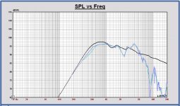
In the plot FFT by Matthias in green, Leap FFT in blue, Leap SPL simulation in black. I used Bagby bafflestep simulation now.
Also 1.5 dB added in Leap. No smoothing with the Leap FFT, you can see the discrete frequency steps below 1 kHz, if you look well.
For some reason we have different FFT results. At this time I start trusting the measurement more... and that the bafflestep simulation makes some errors
Maybe a SPL measurement at 50 cm to get a little longer anechoic FFT window? Just to see. But we have to be aware that bafflestep boost is decreasing closer to the cabinet also.
I thought you had a 192 kHz measurement system?
Edit: I was wondering why does your FFT start only above 300 Hz and not lower?
Attachments
Last edited:
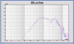
Comparing now in the plot, the in cabinet measurement (FFT with Leap) (blue) with the Volt infinite baffle model, based on measured TSP (pink).
I think this measurement is correct. The cone models used for bafflestep simulations are more directional around 500 to 1000 Hz. The 3 inch midrange dispersion is wider than the driver models. I am almost sure of that, Augerpro also mentioned this.
I think I can check this with a DI calculation out of the off axis measurements and compare with DI out of the driver models.
I will do later.
Edit: I also looked to FFT's with longer gate time, non-anechoic. That is really not correct, the unsmoothed FFT becomes very noisy and smoothing that, that is the wrong way.
IMO we can splice now around 200 Hz for the midrange, starting with that one now. And maybe check the measurements later with a longer gate time if possible.
Attachments
Last edited:
I see your sample frequency is 44 kHz.
It is 44100 Hz. I normaly only use higher sampling rates when it's necessary to capture frequencies above 20 kHz.
I understand your FFT window has to stop at 6 ms, for anechoic response. So you have only a 3 ms impulse duration for FFT.
I did the FFT also in Leap up to 6 ms and I have a different result between 300 and 600 Hz.
I am a bit confused about this now. The setup in the workshop was such that the anechoic part after the main impulse is about 3 ms long (maybe even a bit less). So you should use only the data that starts at with the impulse and ends 3 ms later. The lowest frequency value you get from this 1/3ms = 333 Hz. There is no way to extract lower frequency components. Using a longer time gate (6ms) means you're getting the echoes into the FFT, which you don't want.
For some reason we have different FFT results.
Did you use a windowing function? In my opinion, windowing is a great tool with static signals (for instance for distortion analysis from a sequence of a sine signal). However, for non-static signal like an impulse resonse, it can be tricky. With a perfect dirac signal, the windowing would not do anything (as long as the window maximum is aligned with dirac pulse). With real-world impulse responses that extend over some period of time, the window will start "eroding" the tail of the impulse, and it will do this more and more for the later parts of the impulse response. This means the window function "eats away" the low frequency components, which tend to extend more towards the end of the window function. The higher frequencies are usually focussed in the early part of the impulse response and are therefore hardly affected by the window function. This means the window function attenuates the low-frequency part of the SPL curve, and it does that in a somewhat unpredictable way, because the effect depends on the shape/tail of the impulse response. I therefore prefer to not use windowing (or use a "rectangular" window, which means the same thing as "time gating only").
Also, maybe the longer time gate you used has some undesired effects on your FFT result, because it includes some of the echoes (see above).
IMO we can splice now around 200 Hz for the midrange ... And maybe check the measurements later with a longer gate time if possible.
With the current measurement data you cannot get anechoic SPL down to 200 Hz (see above). In my naive way of looking at this, I'd use the 700-800 Hz overlap between the farfield and nearfield measurements for splicing. As augerpro mentioned, that's where the farfield curve starts to fall off, and the two curves seem to do the same thing in this frequency range.
I was checking out the garden this afternoon for a possible measurement-tower construction site. My family thinks I am going nuts. I have to say they have a point
Last edited:
I only use the reflections free part of the impulse. With 6 ms I mean the absolute time of the impulse measurement or 3 ms impulse data without echos. Indeed, using longer gate times is not correct.
I don't use a FFT window in Leap, it is even not available. You are right using windows is tricky sometimes, in the Clio I also use only a rectangular window.
I will have a closer look at the splicing point. But 700 - 800 Hz is not good in this case, because the baffle step error by the simulation already starts above 200 Hz. It should mean that you have to switch from black to blue (or green) curve in the plot of post 452 at 700 – 800 Hz.
I thought like follows, the SPL below 200 Hz in the simulation is correct and the SPL of the measurement becomes correct in the region 600 Hz and higher. And the SPL between 200 and 600Hz is expected to be a straight line. We don’t have correct SPL values for simulation, neither for measurement between 200 and 600 Hz.
What should be the reason of the SPL difference between the FFT’s at 300 to 600 Hz?
Last edited:
As an information, I had the same bafflestep simulation problem with a 5 inch convex midrange (Usher 0541A) in the Usher BE20 speaker, that I redesigned in the past. Also with that midrange I had no bafflestep boost in the 500 to 1500 Hz region. Also measured in a room using short gate times. I also couldn't explain it at that time.
With that in mind, I am even more convinced that there is a problem with some baffle diffraction simulators, because of wrong cone models.
I have to look for better tools to simulate that in a more correct way... tips are welcome!
With that in mind, I am even more convinced that there is a problem with some baffle diffraction simulators, because of wrong cone models.
I have to look for better tools to simulate that in a more correct way... tips are welcome!
I was checking out the garden this afternoon for a possible measurement-tower construction site. My family thinks I am going nuts. I have to say they have a point
To measure outdoors, I use two stepladders with a shelf in between. That way, the speaker is 1m50 above the ground and the microphone almost 2m. Then I get a gate time of about 8 ms without echos.It is already better than indoors and with the stepladders I don't need to make a tower
.
Last edited:
What should be the reason of the SPL difference between the FFT’s at 300 to 600 Hz?
I am not sure, but my guess is that the longer gate time needed for the lower frequency cut-off in your Leap FFT introduced some signal components from the echoic part that give different SPL in the 300-600 Hz range.
Some of our rooms have a slightly higher ceiling than my workshop/garage, but not very much. If I end up moving everything to a different place, I can also do that outdoors and let my neighbours know that I am nuts.
 Don't hold your breath for that, though.
I am not sure, but my guess is that the longer gate time needed for the lower frequency cut-off in your Leap FFT introduced some signal components from the echoic part that give different SPL in the 300-600 Hz range.
Matthias, I use the same FFT window as you in my Leap FFT.
The impulse starts at about 3ms absolute time and it stops at 6ms absolute time. So the impulse duration is also only 3 ms, available for FFT. I don't use any of the echoic part
.I will try out FFT in REW, if it is possible to import.
Last edited:
- Home
- Loudspeakers
- Multi-Way
- Open Source Monkey Box