Hi,
I posted some application plots of the above to the Horn Honk thread starting from: http://www.diyaudio.com/forums/multi-way/161627-horn-honk-wanted-13.html#post2154285
- Elias
I posted some application plots of the above to the Horn Honk thread starting from: http://www.diyaudio.com/forums/multi-way/161627-horn-honk-wanted-13.html#post2154285
- Elias
Hello,
I did some simple wavelet reassignment to improve the visualisation and to make reflections more emphasisedly visible.
On the left is the wavelet transform of my ideal reflection test impulse response, and on the right is the reassigned wavelet. Amplitude scale is 40dB, colors are as in all of my plots before. Now no problem to identify reflections 😀
An externally hosted image should be here but it was not working when we last tested it.
- Elias
I imagine there is no problem identifing the reflections by looking directly at the impulse response either?

An externally hosted image should be here but it was not working when we last tested it.
In the case of this simple, repeated impulse - no. Easy to see.
But somewhat harder in a measurement of a speaker. The reassigned is handy for that.
But somewhat harder in a measurement of a speaker. The reassigned is handy for that.
I imagine there is no problem identifing the reflections by looking directly at the impulse response either?
One may be able to detect one strong sub 2ms reflection by looking at the impulse response directly, but maybe non of sub 1ms reflections. This is not very good saldo considering the total amount of reflections there is. In the IR the information is squeeched in one bunch, and it's much easier to see the data if you spread it in multiple dimensions (time, amplitude, frequency) like wavelets do.
But hey, if you like to remain looking at the IR plots only, nobody is going to pull you out of your bunker! 😀 Enjoy 🙂
- Elias
Reflections are inherently a time domain phenomena. Regardless of what signal you use for the wavelet fundamentally the wavelet is being convoluted with the impulse. Look at equation 33 or the paper by Ponteggia and Di Cola.
Wh(a, b) = sqrt(a) IFFT [FFT{h(t)} psi(aw)^]
The term in brackets is convolution of the impulse response and the conjugate of the wavelet performed in the frequency domain. The IFFT returns the result to the time domain that is, the result is just h(t)*psi(aw)^ scaled by sqrt(a).
If you are interested in sub 1 msec reflections then the problem is more likely over lapping of the tails of the system impulse with the reflections and their tails. But with a impulse sampled at 48k (0.02 msec between samples) or 96k (0.01 msec between samples) there is still plenty of time resolution there to see closely spaced reflections. You can't get better resolution that you start with from the impulse.
The way to address this is to sharpen the impulse of the reflection free system so that it had a shorter tail. This would reduce or eliminate the over lap so that each spike in the impulse, other than the initial one, would necessarily be a reflection. There is nothing gained by displaying this in TFR format. If done correctly there would be no variation in the F direction, much like your right hand plot (and mine). So what would be the point in extending the representation to TFR when the result is not a function of F? The only case where there would be some variation in the F direction is when the reflections acts as low pass filters, in which case the most detail would be at the lowest frequency and the raw impulse would still be the most revealing. I'm not in a bunker. I just don't think I have to look at esoteric processing to see what is in plane sight. Well, I said all I have to say here so I will now go away.

Last edited:
John, with the skeleton noodles we do exactly the sharpening you are talking about.
And regarding frequency localization - it *is* displayed in wavelet analysis (to out desire) - and much harder to pick in a FR plot .
No one here is arguing that the IR plot is the "full contender" - there are just a lot of analysis / visualizations the excel in one respect or the other .
Michael
And regarding frequency localization - it *is* displayed in wavelet analysis (to out desire) - and much harder to pick in a FR plot .
No one here is arguing that the IR plot is the "full contender" - there are just a lot of analysis / visualizations the excel in one respect or the other .
Michael
I did some simple wavelet reassignment to improve the visualisation and to make reflections more emphasisedly visible.
- Elias
The way to address this is to sharpen the impulse of the reflection free system so that it had a shorter tail. This would reduce or eliminate the over lap so that each spike in the impulse, other than the initial one, would necessarily be a reflection. There is nothing gained by displaying this in TFR format. If done correctly there would be no variation in the F direction, much like your right hand plot (and mine). So what would be the point in extending the representation to TFR when the result is not a function of F? The only case where there would be some variation in the F direction is when the reflections acts as low pass filters, in which case the most detail would be at the lowest frequency and the raw impulse would still be the most revealing.
I think you may have missed the procedure of wavelet reassignment and are talking about something else.
Here's one way to reassign a wavelet, see Chapter 2
http://www.cinc.org/archives/2003/pdf/581.pdf
- Elias
I was wondering, do the skeleton noodles look like DNA fingerprinting strips?
I don't know about "skeleton noodles", but reassignment simulates the same phenoma which formed galaxies of the universe and our solar system too. So they can be called Heavenly Plots 😀
- Elias

Hello,
Not as nice as Elias's noodles or Soogsc's boreal aurora, here attached a "quasi noodles" graph I obtained extracting the local maxima of a quasi wavelets graph.
(E.g. : OLA XT1086 )
Best regards from Paris, France
Jean-Michel Le Cléac'h
Best regards
Not as nice as Elias's noodles or Soogsc's boreal aurora, here attached a "quasi noodles" graph I obtained extracting the local maxima of a quasi wavelets graph.
(E.g. : OLA XT1086 )
Best regards from Paris, France
Jean-Michel Le Cléac'h
Best regards
Attachments
Mige0, have you been able to generate a wavelet yet?
Latest news here :
http://www.diyaudio.com/forums/soft...n-wavelet-analysis-available.html#post2159388
🙂
Michael
It should not be too long till we have enough for an art exhibition.😉
My fist attempt in "heavenly pictures" some days back may come in here handy:
😉

Actually not having had time enough to debug, I stored the pix for its surreal aesthetics.
Seems I didn't get those spaghetti "al dente" yet
😀
Michael
Last edited:
FRs, wavelets, and CSDs of EconoWave Standard and Deluxe:
Flex Your PCD Mettle: - Page 11 - Techtalk at Parts-Express.com
Flex Your PCD Mettle: - Page 11 - Techtalk at Parts-Express.com
Hello,
In order to continue generating the wavelet transform let's jump from here http://www.diyaudio.com/forums/multi-way/164029-wtf-wavelet-transform-audio-measurements-what-how.html#post2145903
This wavelet transform will eventually replace the CSD 😀
The Octave script calculates the transform for you after you enter the parameters. There is no parameters! 😀
Enter only the following:
* impulse response file path and file name (wav file)
* start and stop frequencies
* stop time until you like to see the plot
* amplitude scale you like to see the plot
### ENTER IMPULSE RESPONSE FOLDER PATH
irfolder = 'D:/your_folder/';
### ENTER IMPULSE RESPONSE FILE [.WAV]
irfile = 'your_ir_file.wav';
### ENTER START AND STOP FREQUENCIES [Hz]
fstart = 1000
fstop = 20000
### ENTER STOP TIME
tstop = 0.01
### ENTER PLOT DYNAMIC RANGE [-dB]
dr = -40
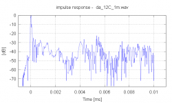
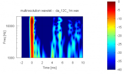
The script generates three plots:
* impulse response plot in dB scale (for convience)
* wavelet transform plot
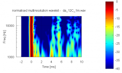
* normalised wavelet transform plot
The code is here:
http://dl.dropbox.com/u/2400456/diyaudio/waveletmultiresoda.m
If you like to try first hand impulse response I'll donate one here:
http://dl.dropbox.com/u/2400456/diyaudio/da_12C_1m.wav
When using the above IR file you should see the plots attached.
- Elias
In order to continue generating the wavelet transform let's jump from here http://www.diyaudio.com/forums/multi-way/164029-wtf-wavelet-transform-audio-measurements-what-how.html#post2145903
This wavelet transform will eventually replace the CSD 😀
The Octave script calculates the transform for you after you enter the parameters. There is no parameters! 😀
Enter only the following:
* impulse response file path and file name (wav file)
* start and stop frequencies
* stop time until you like to see the plot
* amplitude scale you like to see the plot
### ENTER IMPULSE RESPONSE FOLDER PATH
irfolder = 'D:/your_folder/';
### ENTER IMPULSE RESPONSE FILE [.WAV]
irfile = 'your_ir_file.wav';
### ENTER START AND STOP FREQUENCIES [Hz]
fstart = 1000
fstop = 20000
### ENTER STOP TIME
tstop = 0.01
### ENTER PLOT DYNAMIC RANGE [-dB]
dr = -40
The script generates three plots:
* impulse response plot in dB scale (for convience)
* wavelet transform plot
* normalised wavelet transform plot
The code is here:
http://dl.dropbox.com/u/2400456/diyaudio/waveletmultiresoda.m
If you like to try first hand impulse response I'll donate one here:
http://dl.dropbox.com/u/2400456/diyaudio/da_12C_1m.wav
When using the above IR file you should see the plots attached.
- Elias
Attachments
Hello,
Some additional explanations of the previous may be good, so here we go.
The previous post #158 contains the script to calculate a wavelet transform of the impulse response what I call multiresolution wavelet transform. It has the property that the time domain length of the wavelet is fixed at every frequency. This can be seen here:
This type of wavelet transform is comparable to CSD (cumulative spectral decay), but with enhanced resolution in both time and frequency domains.
The calculation essentially sweeps the frequency domain with wavelets envelopes like this:
Then after the repeats at every freq the result is plotted as a color surface.
- Elias
Some additional explanations of the previous may be good, so here we go.
The previous post #158 contains the script to calculate a wavelet transform of the impulse response what I call multiresolution wavelet transform. It has the property that the time domain length of the wavelet is fixed at every frequency. This can be seen here:
An externally hosted image should be here but it was not working when we last tested it.
This type of wavelet transform is comparable to CSD (cumulative spectral decay), but with enhanced resolution in both time and frequency domains.
The calculation essentially sweeps the frequency domain with wavelets envelopes like this:
An externally hosted image should be here but it was not working when we last tested it.
Then after the repeats at every freq the result is plotted as a color surface.
- Elias
It should be noted that there are different wavelet transforms.
The one multiresolution wavelet transform generates this plot from my test impulse response sequence:
The other wavelet transform can be called constant Q wavelet transform, and it has the property that every frequency the wavelets has constant number of cycles. This will generate this plot from the same test impulse response:
The Octave script for constant Q transform in on the way 😀
One selects to use the transform that best suit one's needs in a particular case. Often it's informative to use both of these at the same time to see multible of effects under study.
- Elias
The one multiresolution wavelet transform generates this plot from my test impulse response sequence:
An externally hosted image should be here but it was not working when we last tested it.
The other wavelet transform can be called constant Q wavelet transform, and it has the property that every frequency the wavelets has constant number of cycles. This will generate this plot from the same test impulse response:
An externally hosted image should be here but it was not working when we last tested it.
The Octave script for constant Q transform in on the way 😀
One selects to use the transform that best suit one's needs in a particular case. Often it's informative to use both of these at the same time to see multible of effects under study.
- Elias
- Status
- Not open for further replies.
- Home
- Loudspeakers
- Multi-Way
- WTF!? Wavelet TransForm for audio measurements - What-is? and How-to?