Thanks Alain.
I already do most of the procedure you outlined, but I was most curious how you overlayed the two graphs. Now we know, thanks.
One of the reasons I have extracted detailed xy data from the 12AX7 curves is so I can import this into PSpice Probe and view the manufacturer curves right along with the simulator output. This is the ultimate comparison imo.
The next step for me will be to use PSpice Optimizer which will hopefully optimize the tube model parameters for me. In this sense, I'll be able to create models all from within the PSpice native environment, all I need is detailed curve data and good skeleton paramaterized models, such as Koren's, Rydel's, and Ayumi's.
A model for pentode models design
About what you said for my 6DQ5 curves, this is not a mistake, it is really what I need to see, the screen grid (g2) curves, not the control grid curves (g1) ... And at low g2 voltages, the current is really off the reality. 🙄
But I am almost ready to make my own 6DQ5 model for the "Direct coupled screen grid drive power amp" I am working on because since about two weeks, I work on a pentode model design procedure. I can already have the screen grid contribution working but not the control grid and grids current yet, this is much more complicated and I don't think I will be able to create a complete pentode model before many weeks or months.
Like I said in the other thread "nobody read", I create a special model for designing pentode models and I made my tests on the 6L6GC because there is a lot of graphs for that very popular tube. I generate my first graph tonight :
This is not perfect but I am very happy with the results, for a first try, this is good. I do it fast and my targets choice can be better, I use only currents at a 500V anode voltage to adjust the curves y positions and I adjust the curves slope angle on the last curve, the 50V screen grid current, that's why it is almost perfect ... For my next test, I will adjust the curves y position at a 300V anode voltage and the curves slopes at a 250V screen grid voltage. This way, I think the overall curves will be more accurate.
The first curve at the top, the red 0V curve is also near perfect because it is my "reference curve", every thing else start from that curve. In my design idea, any g1 and g2 voltages can be use for the reference curve, depending where the best accuracy is needed, although the best for g1 is 0V. But like I said, nothing is done yet about the control grid contribution ... 😱
I will not explain here how work my "special pentode model design model" because I don't have time for that but here is where I am in that project, this is the circuit :
The principle is all the needed parameters are passed to the model via the "batteries" voltages ... simple and fast. Here is the model for that "chip looking" pentode symbol :
After all the values are found, I can write a real pentode model with those values, replacing the corresponding V(pins) or written as .PARAM data values. Of course, I still have a lot of work to do in this model but up to now, everything is working well. 😀
I still don't see the images and I find why, my "Comodo Dragon" navigator is blocking the dropbox site ... I get a message saying "Invalid server certificate" and I don't know how to bypass it.You can't see the images? That's weird, may be your ISP/PC is blocking Dropbox? Anyway, I only posted those comparisons to point out that Ayumi models were not so bad when the correct datasheets were used. In any case, I think most of these models should give you good enough indication to see if the circuit will work or not, perhaps just not in the extreme low V/I area that your particular design requires. Direct-coupled screen drive power amp, that you don't see everyday... 😱
About what you said for my 6DQ5 curves, this is not a mistake, it is really what I need to see, the screen grid (g2) curves, not the control grid curves (g1) ... And at low g2 voltages, the current is really off the reality. 🙄
But I am almost ready to make my own 6DQ5 model for the "Direct coupled screen grid drive power amp" I am working on because since about two weeks, I work on a pentode model design procedure. I can already have the screen grid contribution working but not the control grid and grids current yet, this is much more complicated and I don't think I will be able to create a complete pentode model before many weeks or months.
Like I said in the other thread "nobody read", I create a special model for designing pentode models and I made my tests on the 6L6GC because there is a lot of graphs for that very popular tube. I generate my first graph tonight :
An externally hosted image should be here but it was not working when we last tested it.
This is not perfect but I am very happy with the results, for a first try, this is good. I do it fast and my targets choice can be better, I use only currents at a 500V anode voltage to adjust the curves y positions and I adjust the curves slope angle on the last curve, the 50V screen grid current, that's why it is almost perfect ... For my next test, I will adjust the curves y position at a 300V anode voltage and the curves slopes at a 250V screen grid voltage. This way, I think the overall curves will be more accurate.
The first curve at the top, the red 0V curve is also near perfect because it is my "reference curve", every thing else start from that curve. In my design idea, any g1 and g2 voltages can be use for the reference curve, depending where the best accuracy is needed, although the best for g1 is 0V. But like I said, nothing is done yet about the control grid contribution ... 😱
I will not explain here how work my "special pentode model design model" because I don't have time for that but here is where I am in that project, this is the circuit :
An externally hosted image should be here but it was not working when we last tested it.
The principle is all the needed parameters are passed to the model via the "batteries" voltages ... simple and fast. Here is the model for that "chip looking" pentode symbol :
.SUBCKT PENTODE_TEST A G2 G1 K 1 2 3 4 5 6 7 8 9 10 11 12 13 14 15 16
* Pentode real pins
BAK AK 0 V=URAMP(V(A,K)) ; Anode to cathode voltage
BSG SG 0 V=MAX(V(G2,K),0.001) ; Screen grid voltage
* BCG CG 0 V=V(G1,K) ; Control grid voltage
* Reference curve parameters
BCR CR 0 V=V(8,K) ; Current reference without slope
BSGR SGR 0 V=V(9,K); Screen grid reference voltage
BCGR CGR 0 V=V(10,K); Control grid reference voltage
BSA SA 0 V=V(4,K) ; Reference slope angle DY/DX
BSC SC 0 V=V(6,K) ; Reference slope curve 0.01 to 0.001
* Screen grid voltage contribution
BRSG RSG 0 V=V(SG)/V(SGR) ; Relative screen grid voltage to reference
BSGE1 SGE1 0 V=V(3,K) ; Screen grid contribution exponent 1
BSGE2 SGE2 0 V=V(5,K) ; Screen grid contribution exponent 2
BSGC SGC 0 V=(V(RSG)^V(SGE1)*V(CR)+V(RSG)^V(SGE2)*V(CR))/2 ; Contribution
* Control grid voltage contribution
* Anode current calculations
BCP CP 0 V=V(SGC) ; Curve position (No control grid contribution yet)
BRCP RCP 0 V=V(CP)/V(CR) ; Relative curve position to reference current
* Anode current curve slope
BACE ACE 0 V=V(7,K) ; Slope angle correction exponent
BAC AC 0 V=V(RCP)^V(ACE) ; Slope angle correction
BSL SL 0 V=1+V(SA)^V(AC)*TANH(V(AK)*V(SC)); Slope
* Anode current knee
BKS KS 0 V=V(1,K) ; Knee sharpness
BKP KP 0 V=V(2,K)*V(CR)/V(CP); Knee position
BKN KN 0 V=TANH(V(AK)^V(KS)*(V(KP))); Knee
* Anode current
B1 A K I=V(CP)*V(KN)*V(SL)
* Screen grid current calculations
* Control grid current calculations
* Other characteristics
.ENDS
After all the values are found, I can write a real pentode model with those values, replacing the corresponding V(pins) or written as .PARAM data values. Of course, I still have a lot of work to do in this model but up to now, everything is working well. 😀
Last edited:
You are welcome. 🙂Thanks Alain.
I already do most of the procedure you outlined, but I was most curious how you overlayed the two graphs. Now we know, thanks.
One of the reasons I have extracted detailed xy data from the 12AX7 curves is so I can import this into PSpice Probe and view the manufacturer curves right along with the simulator output. This is the ultimate comparison imo.
The next step for me will be to use PSpice Optimizer which will hopefully optimize the tube model parameters for me. In this sense, I'll be able to create models all from within the PSpice native environment, all I need is detailed curve data and good skeleton paramaterized models, such as Koren's, Rydel's, and Ayumi's.
I know the Andrei Frolov "curve captor" can be used to get the triodes X,Y data but I am not a PSpice user and I don't know what can be done with this software. I should verify if I can import x,y data in SiMetrix to output the curves ... There still are many things I don't know about this software. But I currently use MS Excel spreadsheets for my work with coordinate points and math formulas, this software also make graphs from the calculated data. 😉
About what you said for my 6DQ5 curves, this is not a mistake, it is really what I need to see, the screen grid (g2) curves, not the control grid curves (g1) ... And at low g2 voltages, the current is really off the reality. 🙄
But I am almost ready to make my own 6DQ5 model for the "Direct coupled screen grid drive power amp" I am working on because since about two weeks, I work on a pentode model design procedure. I can already have the screen grid contribution working but not the control grid and grids current yet, this is much more complicated and I don't think I will be able to create a complete pentode model before many weeks or months.
Like I said in the other thread "nobody read", I create a special model for designing pentode models and I made my tests on the 6L6GC because there is a lot of graphs for that very popular tube. I generate my first graph tonight :
After all the values are found, I can write a real pentode model with those values, replacing the corresponding V(pins) or written as .PARAM data values. Of course, I still have a lot of work to do in this model but up to now, everything is working well. 😀
I see now WRT 6DQ5, you are using the screen not the grid as the input, then in that case, it would be better not to use the Ayumi model.
Really like what you have managed to create, the result with the 6L6 is quite impressive, looking forward to see more models. 😛
Microcat / LTspice differences
I have taken first steps with uTracer and Reefman's excelent ExtractModel modelling tool. I measured and modeled Siemens RS1019 beam tetrode. It however took several hours to get the model working correctly under Microcap. After hammering head to wall I found the cause. LTspice and Microcap have different definition for LOG() function. Clip from the help files bellow.
LTSpice
__________________________________
ln(x)
Natural logarithm of x
log(x)
Alternate syntax for ln()
log10(x)
Base 10 logarithm
sqrt(x)
Real part of the square root of x, e.g., sqrt(-1) returns 0, not 0.707107i
Microcap
__________________________________
LN(z) Natural Log
LOG(z) Common log
LOG10(z)Common log
SQRT(z) Complex square root of z
__________________________________
After changing LOG to LN Microcap calculations started to be correct. I found also other difference the SQRT() function. I do not have correction for this issue. Maybe SQRT() never gets negative argument because it seems to to cause any problems.
If somebody is interested the RS1019 models and uTracer files are attached. Tube is measured so that both halves are connected together. This is because both sides have common screen grid and my intention is to use two of these tubes in UL PP connection.
From the zip package you can find the .cir files for the LTspice and .ckt files for the Microcap. Also uTracer measurements .bmp pictures are included as well as ExtractModel produced .plt files.
And of cource any comments are welcome.
Attachments
You are welcome. 🙂
I know the Andrei Frolov "curve captor" can be used to get the triodes X,Y data but I am not a PSpice user and I don't know what can be done with this software. I should verify if I can import x,y data in SiMetrix to output the curves ... There still are many things I don't know about this software. But I currently use MS Excel spreadsheets for my work with coordinate points and math formulas, this software also make graphs from the calculated data. 😉
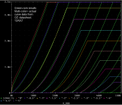
I have yet to compare modeling in Curvecaptor with a few data points vs. with many data points, but I prefer to generate many. With many points, they can be imported into PSpice Probe and compared to the sim results directly. See the attached example. Green is the sim results and multi-colored curves are the actual data off the GE datasheet, extracted with Dagra using Bezier curves.
Note, the example sim model was not generated in Curvecaptor, it is from the EXCEM library.
I don't know if SiMetrix can import data, but it would be nice if it could so you can do the same.
Attachments
Last edited:
I choice the Ayumi model because they are the only one with a grid curve current look like a real grid curve current ... Most of the model from other authors just have a linear current at any anode voltage but the grid current suppose to raise very high when the anode current is dropping, like a "inverse knee" at the same anode voltage. The fact is the screen grid start to act like an anode when the anode current start to drop, that's the way I see it.I see now WRT 6DQ5, you are using the screen not the grid as the input, then in that case, it would be better not to use the Ayumi model.
Really like what you have managed to create, the result with the 6L6 is quite impressive, looking forward to see more models. 😛
Not many people design screen grid drive amplifier because not many tubes are suitable for that, the tube current must be able to be controlled by a very low screen grid voltage so it can work with a 0V control grid voltage without exceeding the maximum anode dissipation. I test all the power pentode and beam power from Ayumi I have in my library and I found many tube suitable for that use :
6BM8, 6CB5, 6CD6, 6CW5, 6DQ5, 6GB5, 6GB8, 6GY5, 6JE6, 6JG6A, 6JR6, 6JS6, 6KD6, 6KM6, 6KV6, 6LF6, 6LG6 and 6146B.
There must be many other but most of these tubes was made for "horizontal-deflection" in television receivers. Some look very good for that application but are more expensive than the 6DQ5. The 6CW5, 6GB5 and 6KM6 are also cheap. 🙂
Thanks to you,I have yet to compare modeling in Curvecaptor with a few data points vs. with many data points, but I prefer to generate many. With many points, they can be imported into PSpice Probe and compared to the sim results directly. See the attached example. Green is the sim results and multi-colored curves are the actual data off the GE datasheet, extracted with Dagra using Bezier curves.
Note, the example sim model was not generated in Curvecaptor, it is from the EXCEM library.
I don't know if SiMetrix can import data, but it would be nice if it could so you can do the same.
You arouse my curiosity and I learn a new think about SiMetrix ... Yes it can import and export the x,y coordinates of any graphs. In the graphs window menu, there are the items "Copy ASCII Data" and "Paste ASCII Data", to and from a normal ASCII text file ... The format of the data for two curves is as follow :
V(Anode) I(g2=150) I(g2=100)
1 3.7293e-005 3.7302e-005
1.6996997 0.000119897 0.000119945
2.399399399 0.000256199 0.000256342
3.099099099 0.000450225 0.000450545
3.798798799 0.000705162 0.000705755
4.498498498 0.001023681 0.001024646
5.198198198 0.001408093 0.0014095
5.897897898 0.001860431 0.00186228
Etc.
This will be very useful for me, to compare the curves of two versions of a model or a circuit, importing or exporting data to or from any software, particularly the Andrei Frolov curve captor and MS Excel. The titles on the first line can be anything but must be there. The V(...) and I(...) are important if you like to see the real unit of the data. The columns must be separated with spaces and/or tabs.
There was only one problem, when I open a new graph page or window and paste the curves data from a text file to compare them to the simulator generated curves, the simulator open a new graph page ... But I find a trick to get both in the same page, I first generate some curves with the simulator, delete them and then paste the curves from the text files. This way, the simulator always draw the next curves in the same graph page, on top of the curves that are already there ! 😛
P.S. I look at the 12AX7 graph you attach, this is a nice comparing job but the model you have is a quite off the GE datasheet curves ...
Last edited:
P.S. I look at the 12AX7 graph you attach, this is a nice comparing job but the model you have is a quite off the GE datasheet curves ...
[Rant]
While all these techniques for comparing curve capture data vs. the datasheet are interesting and useful, at the end of the day, it is the SPICE model that really matters.
We already know that the datasheets were based on the averages of the tubes off the production line, which in most case WILL NOT match up well with the tubes in our collection (especially for modern production tubes). So no matter how accurate the curve capture data may be, they are not likely to match up with the datasheets, and in fact, the SPICE models made from them, may not be of much use to anyone except for yourselves, since no one else has your tubes.😉
Instead, if we just make the best models possible based on the existing datasheets, then more people will be able to use the models with the understanding that the simulation results are going to be +-20% from the bogey due to manufacturing tolerances and the limitation of modeling, and just leave it at that.
There are of course some exceptions, as there are many tubes without enough data (especially for pentodes and beam tetrodes) to make the models, then actual curve traced data from, for example, uTracer & ExtractModel can be used to make the models.
[/Rant]😀
jazbo,
Perhaps you misunderstood.
What I posted was a comparison between the SPICE model simulation results, and the datasheet curves. Isn't that how we know if our tube SPICE model is close enough for practical use?
Perhaps I missed your point?
Perhaps you misunderstood.
What I posted was a comparison between the SPICE model simulation results, and the datasheet curves. Isn't that how we know if our tube SPICE model is close enough for practical use?
Perhaps I missed your point?
That's great news.Thanks to you,
You arouse my curiosity and I learn a new think about SiMetrix ... Yes it can import and export the x,y coordinates of any graphs. In the graphs window menu, there are the items "Copy ASCII Data" and "Paste ASCII Data", to and from a normal ASCII text file ...
In PSpice Probe, there is an "append" button that allows me to merge the two "dat" files, and as such, I can plot traces from either dat file in the same window. Before I can append a dat file, I have to import the csv data into probe, and it converts the data to the native probe data format in a "dat" file.
So I run the simulation as normal, and I get the sim results. Then I append my datasheet xy data (in dat format) to the existing sim results, and voila, instant comparison!
Yes, I know. As I said, this is a 12AX7 model taken from the EXCEM publication. It is not the best fit, but serves to demonstrate what I am explaining.P.S. I look at the 12AX7 graph you attach, this is a nice comparing job but the model you have is a quite off the GE datasheet curves ...
jazbo,
Perhaps you misunderstood.
What I posted was a comparison between the SPICE model simulation results, and the datasheet curves. Isn't that how we know if our tube SPICE model is close enough for practical use?
Perhaps I missed your point?
No, you got it, I was just rambling because I thought I detected a trend to make "one-off" models based on traced curves from a single sample, that's all. I was probably just over-reacting from too much coffee this morning... 😀)
Not at all jazbo.
We're using the published curves to try and model the average performance. 😉
Besides, I don't have a uTracer, so I have no choice but to use the mfr. curves at this point.
We're using the published curves to try and model the average performance. 😉
Besides, I don't have a uTracer, so I have no choice but to use the mfr. curves at this point.
A fantastic curves digitizer
First, I discover with SiMetrix I can separate the X,Y coordinates with a comma in the text data file, this is the CSV Excel format. I also find out the coordinate points are connected together in the order they are read so they cannot be all mixed ... The y coordinates of different curves can be in parallel columns in the file only if all the X coordinates are the same, if not, they have to be "append" on after the others in the file, so as many curves needed can be in the same file. I also discover when I save a SiMetrix graph file and open it back, the new generated curves are draw in the same graph sheet, not in the new one, so I can reuse the digitized curves graph as many time I like, I don't have to paste the ASCII data every times. 🙄
Now the bad news ... I discover my Andrei Frolov Curve Captor don't work properly anymore, can't find the images files ... 😡
More good news ... I was thinking using the Curve Captor for digitizing all my curves, not only for triodes but also for pentodes, but ... Then I took some time to find a good graph digitizer and I found two when I visit the Luke Miller blog. He explain how to digitize a graph using the ImageJ software with the Figure_Calibration plugin. I download the Windows 32 bits with Java version and the plug-in and I found out this is a very powerful image processor software but I don't have time to try it yet, it don't look very "friendly user" ("convivial" in my native language).
But at the end of is blog article, he mention a useful "online digitizer", the WebPlotDigitizer made by Ankit Rohatgi ... I try it and this is a really fantastic tool, allowing digitizing any curves graph very fast and easily. And guest what ... this tool don't have to be used "online", it also work very well "offline". I save the "finish" HTML page on a hard disk drive and I can use in "Manual Mode" without any problems, I don't try the "Automatic Mode", I believe it is just a useless complicated gadget. 😀
A fantastic curves digitizer
When you click on the "Launch" button, this page appear, you can drag and drop the image file you like on it, a first useful feature :
The first thing to do is pressing the "Define Axes" button, then you will have to mark four points on the graph to set the X,Y axes limits, so the graph don't have to be perfectly straight ... Then you will have to enter the limits coordinate values, in my example, it is 700V for the X axis and 400mA for the Y axis, but don't be stupid like me, the first time, I write 400 and I get a 400A high graph ... you have to write 0.4 for 400mA. 😛
As you can see, I put much more points where the curve change a lot, in the straight parts of the curve, just few of them are sufficient. But if you make a mistake, you can easily delete all the last points you like using the "Undo" button. The magnifier window in the top right corner is very useful for accurate positioning of the points.
When the curve is finish, just click the "Create .CSV" button to get the above window, then click on "Select All" and copy (Ctrl C) paste (Ctrl V) the coordinate in your text file. I prepare my text file this way, ready for all the curves all will copy to :
Notice I already write the 0,0 coordinate where every curves begin, so it is always precisely there and I don't have to put a mark for that point on the graph.
It is time now for the second curve, as you can see, I put a mark before every curve begin, so I just have to remove the unneeded marks with the "Undo" button and start from there for the next curve and so on :
The 350V curve is now finish, as you can see, the first seven marks are also common to the 400V curve, this is a time saving method of working. After all curves are done, I copy paste the ASCII data of my text file in the SiMetrix graph window and save it for future uses.
I select all the digitized curves and highlight them to be able to compare them easily to the SiMetrix generated curves from the model I talk about yesterday on this thread preceding page. This is a much faster way to work than "superposing" the SiMetrix graph on the company graph because there is no need to measure the number of pixels of those graphs and adjusting the window size to fit them, the results are very close ... 😉
I got many news tonight,That's great news.
In PSpice Probe, there is an "append" button that allows me to merge the two "dat" files, and as such, I can plot traces from either dat file in the same window. Before I can append a dat file, I have to import the csv data into probe, and it converts the data to the native probe data format in a "dat" file.
So I run the simulation as normal, and I get the sim results. Then I append my datasheet xy data (in dat format) to the existing sim results, and voila, instant comparison!
Yes, I know. As I said, this is a 12AX7 model taken from the EXCEM publication. It is not the best fit, but serves to demonstrate what I am explaining.
First, I discover with SiMetrix I can separate the X,Y coordinates with a comma in the text data file, this is the CSV Excel format. I also find out the coordinate points are connected together in the order they are read so they cannot be all mixed ... The y coordinates of different curves can be in parallel columns in the file only if all the X coordinates are the same, if not, they have to be "append" on after the others in the file, so as many curves needed can be in the same file. I also discover when I save a SiMetrix graph file and open it back, the new generated curves are draw in the same graph sheet, not in the new one, so I can reuse the digitized curves graph as many time I like, I don't have to paste the ASCII data every times. 🙄
Now the bad news ... I discover my Andrei Frolov Curve Captor don't work properly anymore, can't find the images files ... 😡
More good news ... I was thinking using the Curve Captor for digitizing all my curves, not only for triodes but also for pentodes, but ... Then I took some time to find a good graph digitizer and I found two when I visit the Luke Miller blog. He explain how to digitize a graph using the ImageJ software with the Figure_Calibration plugin. I download the Windows 32 bits with Java version and the plug-in and I found out this is a very powerful image processor software but I don't have time to try it yet, it don't look very "friendly user" ("convivial" in my native language).
But at the end of is blog article, he mention a useful "online digitizer", the WebPlotDigitizer made by Ankit Rohatgi ... I try it and this is a really fantastic tool, allowing digitizing any curves graph very fast and easily. And guest what ... this tool don't have to be used "online", it also work very well "offline". I save the "finish" HTML page on a hard disk drive and I can use in "Manual Mode" without any problems, I don't try the "Automatic Mode", I believe it is just a useless complicated gadget. 😀
A fantastic curves digitizer
When you click on the "Launch" button, this page appear, you can drag and drop the image file you like on it, a first useful feature :
An externally hosted image should be here but it was not working when we last tested it.
The first thing to do is pressing the "Define Axes" button, then you will have to mark four points on the graph to set the X,Y axes limits, so the graph don't have to be perfectly straight ... Then you will have to enter the limits coordinate values, in my example, it is 700V for the X axis and 400mA for the Y axis, but don't be stupid like me, the first time, I write 400 and I get a 400A high graph ... you have to write 0.4 for 400mA. 😛
As you can see, I put much more points where the curve change a lot, in the straight parts of the curve, just few of them are sufficient. But if you make a mistake, you can easily delete all the last points you like using the "Undo" button. The magnifier window in the top right corner is very useful for accurate positioning of the points.
An externally hosted image should be here but it was not working when we last tested it.
When the curve is finish, just click the "Create .CSV" button to get the above window, then click on "Select All" and copy (Ctrl C) paste (Ctrl V) the coordinate in your text file. I prepare my text file this way, ready for all the curves all will copy to :
V I(400V)
0,0
4.5103092783505145,0.005405405405405406
12.628865979381443,0.01981981981981982
18.943298969072156,0.04054054054054054
28.865979381443285,0.08468468468468468
37.88659793814433,0.12792792792792793
45.10309278350513,0.16666666666666666
56.82989690721647,0.21981981981981985
71.26288659793815,0.2891891891891892
75.77319587628864,0.30360360360360367
82.08762886597934,0.3171171171171171
91.10824742268042,0.32342342342342345
108.24742268041237,0.3297297297297298
129.8969072164948,0.33513513513513515
164.17525773195874,0.3405405405405406
212.88659793814432,0.34594594594594597
288.659793814433,0.3540540540540541
385.180412371134,0.36036036036036034
551.159793814433,0.3693693693693693
V I(350V)
0,0
V I(300V)
0,0
V I(250V)
0,0
V I(200V)
0,0
V I(150V)
0,0
V I(100V)
0,0
V I(50V)
0,0
Notice I already write the 0,0 coordinate where every curves begin, so it is always precisely there and I don't have to put a mark for that point on the graph.
An externally hosted image should be here but it was not working when we last tested it.
It is time now for the second curve, as you can see, I put a mark before every curve begin, so I just have to remove the unneeded marks with the "Undo" button and start from there for the next curve and so on :
An externally hosted image should be here but it was not working when we last tested it.
The 350V curve is now finish, as you can see, the first seven marks are also common to the 400V curve, this is a time saving method of working. After all curves are done, I copy paste the ASCII data of my text file in the SiMetrix graph window and save it for future uses.
An externally hosted image should be here but it was not working when we last tested it.
I select all the digitized curves and highlight them to be able to compare them easily to the SiMetrix generated curves from the model I talk about yesterday on this thread preceding page. This is a much faster way to work than "superposing" the SiMetrix graph on the company graph because there is no need to measure the number of pixels of those graphs and adjusting the window size to fit them, the results are very close ... 😉
Same for me, I don't have a uTracer Curves Tracer but this is a very interesting system, the only things I don't like about it is the 300V anode and screen grid limitation and there is no positive voltage and current measurement for the control grid. 🙄Not at all jazbo.
We're using the published curves to try and model the average performance. 😉
Besides, I don't have a uTracer, so I have no choice but to use the mfr. curves at this point.
Our friend Yves Monmagnon also design an interesting Tubes Curves Tracer but it don't use "pulsed" high voltages, just the AC 50 Hz (Europa) line variation, clever ... But I don't know if the software for it is working well ? 🙂
Last edited:
uTracer v.4 will overcome those limitations, can't wait for it to be released... As for Yves' tracer, I built one and the circuit worked just fine, however, I could not get the software to work and he no longer (or ever) supports it.
uTracer v.4 will overcome those limitations, can't wait for it to be released... As for Yves' tracer, I built one and the circuit worked just fine, however, I could not get the software to work and he no longer (or ever) supports it.
I have some concerns about the uTracer conceptual implementation, posted here. Appreciate any comment there.
12BY7
Can someone help me make this macro compatible with Tina? I think it takes PSpice, but I don't know the difference. Thanks.
*
* Generic pentode model: 12BY7A
* Copyright 2003--2008 by Ayumi Nakabayashi, All rights reserved.
* Version 3.10, Generated on Fri Dec 27 09:04:07 2013
* Plate
* | Screen Grid
* | | Control Grid
* | | | Cathode
* | | | |
.SUBCKT 12BY7A P G2 G1 K
BGG GG 0 V=V(G1,K)+0.65943158
BM1 M1 0 V=(0.012147484*(URAMP(V(G2,K))+1e-10))**-0.63410138
BM2 M2 0 V=(0.70287195*(URAMP(V(GG)+URAMP(V(G2,K))/24.460049)))**2.1341014
BP P 0 V=0.0067627064*(URAMP(V(GG)+URAMP(V(G2,K))/34.80015))**1.5
BIK IK 0 V=U(V(GG))*V(P)+(1-U(V(GG)))*0.0039175034*V(M1)*V(M2)
BIG IG 0 V=0.0033813532*URAMP(V(G1,K))**1.5*(URAMP(V(G1,K))/(URAMP(V(P,K))+URAMP(V(G1,K)))*1.2+0.4)
BIK2 IK2 0 V=V(IK,IG)*(1-0.4*(EXP(-URAMP(V(P,K))/URAMP(V(G2,K))*15)-EXP(-15)))
BIG2T IG2T 0 V=V(IK2)*(0.82100762*(1-URAMP(V(P,K))/(URAMP(V(P,K))+10))**1.5+0.17899238)
BIK3 IK3 0 V=V(IK2)*(URAMP(V(P,K))+5958)/(URAMP(V(G2,K))+5958)
BIK4 IK4 0 V=V(IK3)-URAMP(V(IK3)-(0.0036749321*(URAMP(V(P,K))+URAMP(URAMP(V(G2,K))-URAMP(V(P,K))))**1.5))
BIP IP 0 V=URAMP(V(IK4,IG2T)-URAMP(V(IK4,IG2T)-(0.0036749321*URAMP(V(P,K))**1.5)))
BIAK P K I=V(IP)+1e-10*V(P,K)
BIG2 G2 K I=URAMP(V(IK4,IP))
BIGK G1 K I=V(IG)
* CAPS
CGP G1 P 0.063p
CGK G1 K 6p
C12 G1 G2 4p
CPK P K 3.5p
.ENDS
From first glance, change ** back to ^.
Works just fine here. Tina understands PSpice and 3f4 spice. 🙂
Code:
*
* Generic pentode model: 12BY7A
* Copyright 2003--2008 by Ayumi Nakabayashi, All rights reserved.
* Version 3.10, Generated on Sat Mar  8 22:41:15 2008
*              Plate
*              | Screen Grid
*              | |  Control Grid
*              | |  |  Cathode
*              | |  |  |
.SUBCKT 12BY7A A G2 G1 K
BGG   GG   0 V=V(G1,K)+-0.02185341
BM1   M1   0 V=(0.014593712*(URAMP(V(G2,K))+1e-10))^-0.7027291
BM2   M2   0 V=(0.68097344*(URAMP(V(GG)+URAMP(V(G2,K))/21.860549)))^2.2027291
BP    P    0 V=0.0061475247*(URAMP(V(GG)+URAMP(V(G2,K))/32.101912))^1.5
BIK   IK   0 V=U(V(GG))*V(P)+(1-U(V(GG)))*0.0036081888*V(M1)*V(M2)
BIG   IG   0 V=0.0030737623*URAMP(V(G1,K))^1.5*(URAMP(V(G1,K))/(URAMP(V(A,K))+URAMP(V(G1,K)))*1.2+0.4)
BIK2  IK2  0 V=V(IK,IG)*(1-0.4*(EXP(-URAMP(V(A,K))/URAMP(V(G2,K))*15)-EXP(-15)))
BIG2T IG2T 0 V=V(IK2)*(0.82512147*(1-URAMP(V(A,K))/(URAMP(V(A,K))+10))^1.5+0.17487853)
BIK3  IK3  0 V=V(IK2)*(URAMP(V(A,K))+4890)/(URAMP(V(G2,K))+4890)
BIK4  IK4  0 V=V(IK3)-URAMP(V(IK3)-(0.0033632383*(URAMP(V(A,K))+URAMP(URAMP(V(G2,K))-URAMP(V(A,K))))^1.5))
BIP   IP   0 V=URAMP(V(IK4,IG2T)-URAMP(V(IK4,IG2T)-(0.0033632383*URAMP(V(A,K))^1.5)))
BIAK  A    K I=V(IP)+1e-10*V(A,K)
BIG2  G2   K I=URAMP(V(IK4,IP))
BIGK  G1   K I=V(IG)
* CAPS
CGA   G1  A  0.063p
CGK   G1  K  6.1p
C12   G1  G2 4.1p
CAK   A   K  3.4p
.ENDS- Home
- Amplifiers
- Tubes / Valves
- Vacuum Tube SPICE Models