There is not another low frequency sine for all that the sample points look like there should be....Ok when you going on on discrete domain you have infinite images positioned on k*fs+fo k*fs-fo
But on my simulation i obtain the samples describing
another sine at low frequencies no aliasing is possible
because fo is inside fc/2 .
Fo is inside Fs/2 , but Fs +-Fo is not inside Fs/2, neither is 2Fs+-Fo, or any of the others that you implicitly created when you sampled at discreet points....
Ok, look forget about sampling, discreet time systems, all that stuff, lets just play with some continuous time sine waves.
Let w1 = 2 * Pi * 999
let w2 = 2 * Pi * 1001
Then sin (w1 t) = 999Hz sine wave, and sin (w2 t) = 1001hz sine wave, nothing to see here.....
Right, now sum them:
sin (w1 t) + sin (w2 t)
Now you get something which very much like what you were seeing, which is no surprise as sin (a) + sin (b) = 2 sin ((a+b)/2) cos ((a - b)/2) which is to say that two sine waves are equivalent to a single sine wave at the average frequency amplitude modulated by a cosine at half the difference frequency, to nobody who has ever built a simple radios surprise (Think double sideband suppressed carrier modulation).
This applies to sampling because you have your sample points representing the baseband sine plus all of the other image sine waves, seriously apply a reconstruction filter and it all just works.
Reconstruction is not just joining the dots, it is not even joining the dots with splines, it is joining the dots in the single, unique manner that is possible within the constraint that all frequencies fall below Fs/2.
Regards, Dan.
In my PC I have RAID. The harddisks rotate at slightly different speeds, so the noise that comes out of the PC is exactly what you'd expect from the sum of two sines of close frequency : vvvvrrrrRRRRRRRrrrrrrvvvvvvvvvrrrrrRRRRRRR, quite annoying btw.
Also, when testing a DAC with square waves, remember, it is like in the Matrix, there is no square wave.
When you see a square wave with wiggly bits on the corners on your scope, it isn't because the DAC added the wiggly bits, it is because it removed the higher harmonics that make the corners square.
If you want your square corners a bit more round and less wiggly, you need to acquire your analog signal at higher Fs and with a more gentle filter (ie, remove a bit more low order harmonics, let through a bit more high order, and add a bit of phase lag). If your signal was already acquired at 44k then bummer, you'll need to throw away the upper octave to get your gentle rolloff (just like NonOS does, except NonOS also adds tons of HF crap).
A DAC that has good looking response on say, a 10k square wave af 44k Fs, without wiggly corners, isn't doing proper reconstruction, it is doing artistic reinterpretation on the signal, like a tone control, nothing wrong with that as long as you like the sound...
Last edited:
Sinc on recostruction filter
tc=time of samplerate
k= integer
2*3.14159*15000 = angular velocity of pulsation in rad/sec
On octave
k=1:341
tc=1/44100
xt=sine(2*3.14159*15000*k*tc)
plot (k,xt)
If you divide properly the samples of this example you
can find another tone we call it fd .
Ok fd have the two images -fx +fx not in phase but at the
same amplitude .
It is inexplicable by your solution because you don't have appreciable error on Calculus as sine as nearest as the same sine .
I have try it on many programs but the modulation is present .
By hand the calculus is not simple to demonstrate but i found the points were is the minimums interactions .
That is placed on fc/9 fc/6 and fc/3 .
It's not a beat but a cyclostationary process to produce a
wave modulated .
I the example sinc is not present , but
I'm sure the spline of over sampling pass trough the original samples , this means I auditioning a noise
at low frequencies of the valid band
There is not another low frequency sine for all that the sample points look like there should be....
Fo is inside Fs/2 , but Fs +-Fo is not inside Fs/2, neither is 2Fs+-Fo, or any of the others that you implicitly created when you sampled at discreet points....
Ok, look forget about sampling, discreet time systems, all that stuff, lets just play with some continuous time sine waves.
Let w1 = 2 * Pi * 999
let w2 = 2 * Pi * 1001
Then sin (w1 t) = 999Hz sine wave, and sin (w2 t) = 1001hz sine wave, nothing to see here.....
Right, now sum them:
sin (w1 t) + sin (w2 t)
Now you get something which very much like what you were seeing, which is no surprise as sin (a) + sin (b) = 2 sin ((a+b)/2) cos ((a - b)/2) which is to say that two sine waves are equivalent to a single sine wave at the average frequency amplitude modulated by a cosine at half the difference frequency, to nobody who has ever built a simple radios surprise (Think double sideband suppressed carrier modulation).
This applies to sampling because you have your sample points representing the baseband sine plus all of the other image sine waves, seriously apply a reconstruction filter and it all just works.
Reconstruction is not just joining the dots, it is not even joining the dots with splines, it is joining the dots in the single, unique manner that is possible within the constraint that all frequencies fall below Fs/2.
Regards, Dan.
tc=time of samplerate
k= integer
2*3.14159*15000 = angular velocity of pulsation in rad/sec
On octave
k=1:341
tc=1/44100
xt=sine(2*3.14159*15000*k*tc)
plot (k,xt)
If you divide properly the samples of this example you
can find another tone we call it fd .
Ok fd have the two images -fx +fx not in phase but at the
same amplitude .
It is inexplicable by your solution because you don't have appreciable error on Calculus as sine as nearest as the same sine .
I have try it on many programs but the modulation is present .
By hand the calculus is not simple to demonstrate but i found the points were is the minimums interactions .
That is placed on fc/9 fc/6 and fc/3 .
It's not a beat but a cyclostationary process to produce a
wave modulated .
I the example sinc is not present , but
I'm sure the spline of over sampling pass trough the original samples , this means I auditioning a noise
at low frequencies of the valid band
You are plotting discreet time points on the wave and joining the dots with straight lines, THAT DOES NOT WORK, it is not how any sane DAC works!
You have to lowpass filter to get the continuous time reconstruction, not linear interpolate, or spline fit or anything else, LOW PASS FILTER.
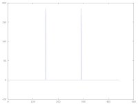
plot (k,fft(xt)) {scilab} will show you the two components in the frequency domain, note what happens as your frequency approaches Fs/2 (the middle of the horizontal axis).
That upper spike is the lower sideband of the first image.
Incidentally, k=1:441 makes reading out frequencies in the fft easy.
Regards, Dan.
You have to lowpass filter to get the continuous time reconstruction, not linear interpolate, or spline fit or anything else, LOW PASS FILTER.
plot (k,fft(xt)) {scilab} will show you the two components in the frequency domain, note what happens as your frequency approaches Fs/2 (the middle of the horizontal axis).
That upper spike is the lower sideband of the first image.
Incidentally, k=1:441 makes reading out frequencies in the fft easy.
Regards, Dan.
Your waves
Triangle wave have 3 orders on Fourier transfer so high
Square wave have 5 orders on Fourier transfer so high
If they have a 10khz of fo on spectrum analysis you find
20Khz 30khz etc...
Over about 20Khz you have Aliasing effect
Answer my question first and I'll get to your stuff.
Triangle wave have 3 orders on Fourier transfer so high
Square wave have 5 orders on Fourier transfer so high
If they have a 10khz of fo on spectrum analysis you find
20Khz 30khz etc...
Over about 20Khz you have Aliasing effect
Low pass filter
Low pass filter can't delete the low frequencies inside samples , for example if low pass filter is ideal positioned at 20Khz the sine at 15KHz pass trough and all sine waves below .
fft on my example there is a "line"(sine tone) at low frequencies .
I have just tryed it and i don't found significant effects
In last istance for CD is not a big problem component over fc/9 have a small amplitude but is a digital noise .
You are plotting discreet time points on the wave and joining the dots with straight lines, THAT DOES NOT WORK, it is not how any sane DAC works!
You have to lowpass filter to get the continuous time reconstruction, not linear interpolate, or spline fit or anything else, LOW PASS FILTER.
plot (k,fft(xt)) {scilab} will show you the two components in the frequency domain, note what happens as your frequency approaches Fs/2 (the middle of the horizontal axis).
That upper spike is the lower sideband of the first image.
Incidentally, k=1:441 makes reading out frequencies in the fft easy.
Regards, Dan.
Low pass filter can't delete the low frequencies inside samples , for example if low pass filter is ideal positioned at 20Khz the sine at 15KHz pass trough and all sine waves below .
fft on my example there is a "line"(sine tone) at low frequencies .
I have just tryed it and i don't found significant effects
In last istance for CD is not a big problem component over fc/9 have a small amplitude but is a digital noise .
If you violate the boundary conditions of the theorem by doing an incorrect reconstruction, you get erroneous results. Your results are erroneous. I'm not sure how many times this needs to be repeated.
You might want to put your spreadsheet away and do the actual experiment with an ordinary ADC/DAC system- when your experiment gives you a different result than your calculation, discard the calculation.
You might want to put your spreadsheet away and do the actual experiment with an ordinary ADC/DAC system- when your experiment gives you a different result than your calculation, discard the calculation.
I have many reasnos but...
Ok i complete understand what do you toking about .
Now i propose you the complete example.
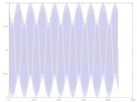
1.Consider a pure sine tone placed at 15KHz this is all
inside fc/2. where fc is sample rate
2.Applying an ideal ADC to the sine uder octave
k=1:441
tc=1/44100
xt=sin(2*3.14159*15000*k*tc)
plot (k,xt)
3. The plot is this
Step 1You are plotting discreet time points on the wave and joining the dots with straight lines, THAT DOES NOT WORK, it is not how any sane DAC works!
You have to lowpass filter to get the continuous time reconstruction, not linear interpolate, or spline fit or anything else, LOW PASS FILTER.
plot (k,fft(xt)) {scilab} will show you the two components in the frequency domain, note what happens as your frequency approaches Fs/2 (the middle of the horizontal axis).
That upper spike is the lower sideband of the first image.
Incidentally, k=1:441 makes reading out frequencies in the fft easy.
Regards, Dan.
Ok i complete understand what do you toking about .
Now i propose you the complete example.
1.Consider a pure sine tone placed at 15KHz this is all
inside fc/2. where fc is sample rate
2.Applying an ideal ADC to the sine uder octave
k=1:441
tc=1/44100
xt=sin(2*3.14159*15000*k*tc)
plot (k,xt)
3. The plot is this
Attachments
Last edited:
next step
2 step
You suggest to applying a fft transform to the sample under octave
plot(k,fft(xt))
The results in the figure are fo and fc-fo only it is right
2 step
You suggest to applying a fft transform to the sample under octave
plot(k,fft(xt))
The results in the figure are fo and fc-fo only it is right
Attachments
Last edited:
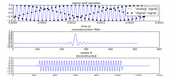
Here ya go.
First I create an "analog" signal (it's just oversampled but that's well enough so it looks pleasing to the eye).
Since it is a pure 15k sine, it is perfectly bandlimited and by sampling it at 44.1k, no information is lost. The samples are the black dots.
It looks like there is a beat frequency, visually.
Note I do not display lines between samples because it makes no sense. Lines should only be displayed when the oversampling is high enough (or the signal slow enough) that linear interpolation doesn't give too much bogus results. Which is obviously not the case here.
The sinc reconstruction brings back the original "analog" signal, as you see. No problem.
Code:
from numpy import *
import matplotlib.pyplot as plt

# create "analog" signal

def make_signal( Fs, NSamples, freq, oversampling ):
	Fs *= oversampling
	NSamples *= oversampling
	t  = arange(NSamples) * (1.0/Fs)
	return t, cos( 2*pi*freq*t )

Fs       = 44100.
NSamples = 100
freq	 = 15000.

plt.figure(1)

plt.subplot(3,1,1)
analog_t, analog_signal = make_signal( Fs,  NSamples, freq, 16 )
plt.plot( analog_t, analog_signal, "b-", label='"analog" signal' )

digital_t, digital_signal = make_signal( Fs,  NSamples, freq, 1 )
plt.plot( digital_t, digital_signal, "ko", label='"digital" signal' )

plt.xlabel("time (s)")
plt.title("signal and samples")
plt.legend()
plt.tight_layout()

plt.subplot(3,1,2)
reconstruct_oversample_ratio = 8
reconstruct_length = 32 * reconstruct_oversample_ratio

impulse = sinc( (1.0/reconstruct_oversample_ratio) * arange( -reconstruct_length, reconstruct_length ) )

plt.plot( impulse )
plt.xlabel("sample #")
plt.title("reconstruction filter")
plt.tight_layout()

plt.subplot(3,1,3)

# recondtruct sampled signal
# first insert zeros
digital_signal_padded = zeros( NSamples * reconstruct_oversample_ratio )
digital_signal_padded[::reconstruct_oversample_ratio] = digital_signal

# then convolve (very dumb method)

reconstructed = convolve( digital_signal_padded, impulse )

plt.plot( reconstructed )
plt.title( "reconstructed" )
plt.show()
Attachments
Last edited:
next step
3 step
On fft is not present the modulation results see step 2 because they
on ideal sample rate the images at dx an sx off zero axis
are in opposition of phase .
But i wont to see them now now we need to separate the samples of +fd and -fd where fd is modulation results .
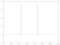
We take a 3k samples on octave
and print out the results on octave
m=3*k
xt=sin(2*3.14159*15000*m*tc)
plot(m,xt)
And results are this
3 step
On fft is not present the modulation results see step 2 because they
on ideal sample rate the images at dx an sx off zero axis
are in opposition of phase .
But i wont to see them now now we need to separate the samples of +fd and -fd where fd is modulation results .
We take a 3k samples on octave
and print out the results on octave
m=3*k
xt=sin(2*3.14159*15000*m*tc)
plot(m,xt)
And results are this
Attachments

Last edited:
fft for the modulation results
Step 4
Now we can plot fft by +fd on octave
plot(m,fft(xt))
the results are this now we can see the modulation
Step 4
Now we can plot fft by +fd on octave
plot(m,fft(xt))
the results are this now we can see the modulation
Attachments
Last edited:
In last
Is possible the two modulations +fd are not exactly in opposition of phase time error on samplerate that means there is a noise. contribution under fc/2 and pass trough the filter
unchanged .
Is possible the two modulations +fd are not exactly in opposition of phase time error on samplerate that means there is a noise. contribution under fc/2 and pass trough the filter
unchanged .
Last edited:
Read what I said. Your issue is images, not aliases.gumo73 said:On Shannon theory you have a aliasing only if signal that you converting from analogue to digital have frequencies or in oder hand components up of fc/2 where fc=Sample rate frequency . On may example the component or all inside this limit
I have already told you that reconstruction filters do not use spline functions.On the reconstruction filter spline pass trough
the original samples
The basic issue is this: how many people need to tell you in how many different ways that you have not understood the need for and the operation of a reconstruction filter before you get it? You could even add such a filter (perhaps a crude one) to your calculations.
If you sample a 15kHz sine wave at 44.1kHz then the principal outputs will be the original signal at 15kHz and the first image at 29.1kHz, at similar amplitudes (the 15 will be slightly bigger). There will also be higher frequency images, at lower amplitudes. As 29.1kHz is almost the second harmonic of 15kHz you will see it adding and subtracting from the peaks to produce what look like beats. If you remove the 29.1kHz, which is exactly what a reconstrction filter does, then you are left with 15kHz. You have two sensible options:
1. convince yourself that this is true by carrying out the full calculation/simulation rather than doing only half a job
or
2. believe us and the textbooks when we tell you that this is true
There are two other options:
3. convince yourself that everyone else is wrong and you have discovered a major flaw in the Shannon sampling theory
or
4. just stay confused
I think we are seeing here the 'Dunning and Kruger effect':
In a given subject area, ignorant people will a) fail to recognize their own ignorance; b) fail to recognize genuine skill in others; c) fail to recognize the extend of their ignorance. 😉
Jan
In a given subject area, ignorant people will a) fail to recognize their own ignorance; b) fail to recognize genuine skill in others; c) fail to recognize the extend of their ignorance. 😉
Jan
thanks for compliments
I think we are seeing here the 'Dunning and Kruger effect':
In a given subject area, ignorant people will a) fail to recognize their own ignorance; b) fail to recognize genuine skill in others; c) fail to recognize the extend of their ignorance. 😉
Jan
Its not a compliment.
BTW What do you think of the post by peufeu above? Doesn't that give you pause to think?
jan
BTW What do you think of the post by peufeu above? Doesn't that give you pause to think?
jan
Complimenrts
Is not certain a place to write certain compliments but only a interchanging opinions in quiet muds
Its not a compliment.
BTW What do you think of the post by peufeu above? Doesn't that give you pause to think?
jan
Is not certain a place to write certain compliments but only a interchanging opinions in quiet muds
Is possible the two modulations +fd are not exactly in opposition of phase time error on samplerate that means there is a noise. contribution under fc/2 and pass trough the filter
unchanged .
And amplitude error on samples can do this sines visible
- Status
- Not open for further replies.
- Home
- Member Areas
- The Lounge
- Shannon ad fc/2 tricks