I have been doing numerous sims of waveguides, and wonder how others are doing. It seems to me that as the sidewall angles get closer to 90deg axisymmetric, then HOMS suddenly start appearing.
I have been doing numerous sims of waveguides, and wonder how others are doing. It seems to me that as the sidewall angles get closer to 90deg axisymmetric, then HOMS suddenly start appearing.
HOMs never "suddenly appear". They are always present, but go lower and lower in frequency as the wall angle widens.
I'm still working on it, but the trend seems like pressure contour look quite smooth until wall angles reach a certain angle, then, like flow separation, the pressure contour lines get real messy. What is interesting is that the on-axis notch also apears as the wall angles widen.HOMs never "suddenly appear". They are always present, but go lower and lower in frequency as the wall angle widens.
I recall Michael was doing some sims using a plane wave source. I kind of wonder what his experience is.
What happens is that the geometry is such that if the aperture is illuminated with a spherical wave Fresnel diffraction results if a second Fresnel zone fits within the aperture.
The appearance of a hole in the middle is good in that it indicates the device is producing what are good spherical wavefronts with a minimum of aperture diffraction.
Rcw.
The appearance of a hole in the middle is good in that it indicates the device is producing what are good spherical wavefronts with a minimum of aperture diffraction.
Rcw.
Shouldn't good spherical wave front also have a very uniform pressure contour? I am a bit confused.
Quite a while back, when I posted this:
http://www.diyaudio.com/forums/showpost.php?p=1590534&postcount=1776
Earl's response was this:
http://www.diyaudio.com/forums/showpost.php?p=1590563&postcount=1777
Looking at polar pressure contour plots, I tend to feel that
Quite a while back, when I posted this:
http://www.diyaudio.com/forums/showpost.php?p=1590534&postcount=1776
Earl's response was this:
http://www.diyaudio.com/forums/showpost.php?p=1590563&postcount=1777
Looking at polar pressure contour plots, I tend to feel that
An externally hosted image should be here but it was not working when we last tested it.
The point that Earl makes is that it is precisely because the wavefront is a very good resemblance to spherical that complete phase cancellation can occur and produce a center minimum.
Up to the point where the wavelength is small enough to admit a second Fresnel zone into the aperture
the wavefront always has a center maximum.
In a device producing a very good spherical wavefront, this has a Gaussian distribution.
What happens is that the wavefront becomes non Gaussian, i.e. develops a central minimum when the wavelength is small enough to admit a second Fresnel zone.
If on the other hand there is a large aperture diffraction field, and the wavefront amplitude more resembles a plane wave, then the wavefront cannot produce a center minimum, ( because the criteria for Fresnel diffraction are not met), and you get a central maximum with a series of minima and maxima on either side.
Rcw.
So how wide a bandwidth can this consistently happen for?The point that Earl makes is that it is precisely because the wavefront is a very good resemblance to spherical that complete phase cancellation can occur and produce a center minimum.
Up to the point where the wavelength is small enough to admit a second Fresnel zone into the aperture
the wavefront always has a center maximum.
In a device producing a very good spherical wavefront, this has a Gaussian distribution.
What happens is that the wavefront becomes non Gaussian, i.e. develops a central minimum when the wavelength is small enough to admit a second Fresnel zone.
If on the other hand there is a large aperture diffraction field, and the wavefront amplitude more resembles a plane wave, then the wavefront cannot produce a center minimum, ( because the criteria for Fresnel diffraction are not met), and you get a central maximum with a series of minima and maxima on either side.
Rcw.
The point that Earl makes is that it is precisely because the wavefront is a very good resemblance to spherical that complete phase cancellation can occur and produce a center minimum.
Rcw.
This is exactly the case and the reason that we seldom see the axial holes with most horns. ONLY when the wavefront at the mouth is very near a pure spherical wavefront can this hole occur.
If this is the case, does this mean we can only hope for a "very near to pure spherical wavefront" in a very small region of the audio spectrum?This is exactly the case and the reason that we seldom see the axial holes with most horns. ONLY when the wavefront at the mouth is very near a pure spherical wavefront can this hole occur.
There are ways of getting around this inherent bandwidth limitation, one curve I have looked at is what I call the “Oskugel”..
This needs a 20mm. Throat driven by a plane wave and has an expansion that is O.S. Until this reaches its Rayleigh length, (where the radius is greater than the throat radius by the square root of two), and a circular arc curve thereafter.
What this essentially does is to give the spherical wavefront a meta-center that moves in such a way as to keep the effective aperture from admitting a second Fresnel zone. It has two transition zones where the wavefront is less than ideal, but close to the best you can achieve if you want a device with good approximations to spherical wavefronts, and c.d., over this bandwidth.
Rcw.
I don't know what frequency range you are showing, but for both types of pressure contours, they seem pretty irregular, I can't understand how this relates to a spherical wave front.
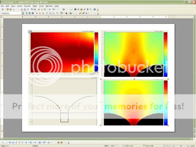
This simulation uses the Axidriver software with a flat 20mm. Piston on an infinite baffle with a bandwidth of 1-20kHz. And a sampling frequency of 44.2kHz.
The -6db. directivity is within +- 3db. Over this bandwidth, and the two plots I have shown are at the two frequencies at around 9.5 and 15.5kHz. Where the glitches appear in the sonogram plot.
These are not the best looking wavefronts the device produces they are the worst, and with this software they seem to be exaggerated somewhat.
A flat 20mm. Piston is used because this is theoretically capable of producing a diffraction interference free beam over this 1-20k. Bandwidth on an infinite baffle, it however does not have constant directivity.
I initially used this to check the software to see if the wavefront amplitude profiles accord with theoretical predictions and they by an large do.
If you want to talk about comparisons between various designs you must compare like with like and thus you must model your design using the same sampler inputs the same graph scale and the same driving piston.
Overall we are not looking to make the nicest picture but trying to see what the gadget is actually doing, and in the cases that I post I have illustrated some of the worst ones, not the prettiest.
Rcw.
My experience with AxiDriver is that the baffled sim curves give a reasonable prediction what the actual device will behave like free standing, below 10KHz, and above the cutoff frequency. I have showed some comparisons in the past.
The problem is that whenever I start to widen the beam, the pressure contours become quite irregular long before 90 deg. So with all the talk about the spherical wave front and HOMs, there seems not enough data to match what is talked about.
I still am under the impression that good wavefront should be associated with uniform pressure contour lines. This is why I am quite curious about the 90deg side walls described here from the beginning.
Last edited:
I'm by no means a theoretical expert but I would think that there is not necessarily a strong mutual correlation between smooth pressure contour plots and the "sphericalness" of wavefront. For the judgement of the wavefront quality we would need to look in the time domain for uniform arrival time of impulse responses vs. angle. If we find, looking from a set of far field distances, a center point (which need not necessarily be the diaphragm center and also might move a little with frequency) this would indicate sphericalness, especially if impulse responses are clean -- only little delayed reflections visible, that is. Still the pressure contour could be irregular to some extent. And vice versa, a clean/smooth contour plot doesn't tell us the wavefront shape directly.. albeit there seem to be indicators for those who can interpret these plots in all subtle details.I still am under the impression that good wavefront should be associated with uniform pressure contour lines.
Just my uneducated 2cts...
- Klaus
If we just look at a single frequency, if it's a sherical wave front, then each equal pressure line should be along a constant radius arc within the expected beam width range. This is what seems reasonable to me. However, in all the simulations performed, it does seems only possible for a quite narrow bandwidth; as the horn wall angles exceed 60 deg approaching 90 deg, things get worse. So I am curiouse...I'm by no means a theoretical expert but I would think that there is not necessarily a strong mutual correlation between smooth pressure contour plots and the "sphericalness" of wavefront. For the judgement of the wavefront quality we would need to look in the time domain for uniform arrival time of impulse responses vs. angle. If we find, looking from a set of far field distances, a center point (which need not necessarily be the diaphragm center and also might move a little with frequency) this would indicate sphericalness, especially if impulse responses are clean -- only little delayed reflections visible, that is. Still the pressure contour could be irregular to some extent. And vice versa, a clean/smooth contour plot doesn't tell us the wavefront shape directly.. albeit there seem to be indicators for those who can interpret these plots in all subtle details.
Just my uneducated 2cts...
- Klaus
It is the isophase surface that is spherical not the isobaric one.
Look at the phase plot in Axidriver.
rcw.
Look at the phase plot in Axidriver.
rcw.
What Soongsc is describing is what I have been saying all along. But at any rate, I don't get the facination with "spherical wavefronts", at least not to the point being discussed here. It's the far field response over a defined bandwidth that matters and nearfield effects don't predict far-field results.
Nothing that anyone has found with all these simulations is anything new as far as I can tell.
Nothing that anyone has found with all these simulations is anything new as far as I can tell.
It is true that trying to get a ninety degree beam with no use of diffraction is pushing it somewhat, a beam can only be truly Gaussian out to around one radian, say sixty degrees.
One thing we do know about the near field and that is that in order for it to have the required far field characteristics it must be a very good approximation to a potential field in order to map to the far field in the way we require.
What I have discovered is that over 1.5-20kHz., with a ninety degree nominal directivity and acceptable near to far field mapping, can just about be done if we use a smaller throat, (i.e. around 20mm.), than the smallest standard compression driver has, and a less than optimal mouth area, (but giving acceptable results with a nominaly ten inch driver).
Basic theoretical considerations tell us this anyway.
Rcw.
Which phase plot are you talking about? Processing a certain curve for minimum phase?It is the isophase surface that is spherical not the isobaric one.
Look at the phase plot in Axidriver.
rcw.
- Home
- Loudspeakers
- Multi-Way
- Geddes on Waveguides