Acoustic Horn Design – The Easy Way (Ath4)

[mabat]

That's indeed a terrible horn.

 

[TNT]

Started an ATH based adventure here: https://www.diyaudio.com/community/threads/hornflower-2-way-point-source.386363/

//

 

[Patrick Bateman]

Does anyone know why my reports do this?

The traces are doubled and there's this weird zig zag pattern.

I have ATH installed on three machines and they all do this.

Here's the config file that produced this:


R-OSSE = {
R = 152 ; [mm]
r0 = 17 ; [mm]
a0 = 10 ; [deg]
a = 34.4836 ; [deg]
k = 1.6226 + 3.4566*abs(sin(p))^2.1429; []
r = 0.32683 ; []
b = 0.13157 ; []
m = 0.81285 ; []
q = 4.011 ; []
}

Source.Contours = {
zoff -2

point p1 4.68 0 2
point p2 0 14 0.5
point p3 1 15 0.5
point p4 0 16 0.5
point p5 0 17 1
cpoint c1 -18.59 0
cpoint c2 0 15

arc p1 c1 p2 1.0
arc p2 c2 p3 0.75
arc p3 c2 p4 0.25
line p4 p5 0
line p5 WG0 0
}

Mesh.LengthSegments = 36
Mesh.AngularSegments = 48
Mesh.ThroatResolution = 5
Mesh.MouthResolution = 9
Mesh.WallThickness = 8
Mesh.RearResolution = 20

Mesh.SubdomainSlices = 35
Mesh.InterfaceOffset = 25
Mesh.InterfaceDraw = 0

ABEC.MeshFrequency = 1000
ABEC.NumFrequencies = 32
ABEC.Abscissa = 1
ABEC.SimType = 2
ABEC.f1 = 500
ABEC.f2 = 12000

ABEC.Polars:SPL_H = {
MapAngleRange = 0,90,19
NormAngle = 0
}

ABEC.Polars:SPL_V = {
MapAngleRange = 0,90,19
NormAngle = 0
Inclination = 90
}

Output.ABECProject = 1
Output.STL = 1

Report = {
PolarData = "SPL_H"
NormAngle = 10
MaxAngle = 90
}

 

[maiky76]

Does anyone know why my reports do this?

The traces are doubled and there's this weird zig zag pattern.

I have ATH installed on three machines and they all do this.

Here's the config file that produced this:


R-OSSE = {
R = 152 ; [mm]
r0 = 17 ; [mm]
a0 = 10 ; [deg]
a = 34.4836 ; [deg]
k = 1.6226 + 3.4566*abs(sin(p))^2.1429; []
r = 0.32683 ; []
b = 0.13157 ; []
m = 0.81285 ; []
q = 4.011 ; []
}

Source.Contours = {
zoff -2

point p1 4.68 0 2
point p2 0 14 0.5
point p3 1 15 0.5
point p4 0 16 0.5
point p5 0 17 1
cpoint c1 -18.59 0
cpoint c2 0 15

arc p1 c1 p2 1.0
arc p2 c2 p3 0.75
arc p3 c2 p4 0.25
line p4 p5 0
line p5 WG0 0
}

Mesh.LengthSegments = 36
Mesh.AngularSegments = 48
Mesh.ThroatResolution = 5
Mesh.MouthResolution = 9
Mesh.WallThickness = 8
Mesh.RearResolution = 20

Mesh.SubdomainSlices = 35
Mesh.InterfaceOffset = 25
Mesh.InterfaceDraw = 0

ABEC.MeshFrequency = 1000
ABEC.NumFrequencies = 32
ABEC.Abscissa = 1
ABEC.SimType = 2
ABEC.f1 = 500
ABEC.f2 = 12000

ABEC.Polars:SPL_H = {
MapAngleRange = 0,90,19
NormAngle = 0
}

ABEC.Polars:SPL_V = {
MapAngleRange = 0,90,19
NormAngle = 0
Inclination = 90
}

Output.ABECProject = 1
Output.STL = 1

Report = {
PolarData = "SPL_H"
NormAngle = 10
MaxAngle = 90
}

Here is what I got.
There are 3 fields for the impedance it might be the issue?

What tweeter did you model?

 

[maiky76]

Probably what you were looking for (normalized to 10deg) and SPL not normalized

 

[mabat]

BTW, it seems that the far off-axis diffraction products in the horizontal plane can be reduced by making the mouth slightly elliptical, i.e. to set the R to something like this:

R = 152 - E*sin(p)^2 ; [mm]
; E = "eccentricity factor" [mm]

 

[mabat]

Probably what you were looking for (normalized to 10deg)

You shouldn't do that, i.e. to normalize both H and V independently to any other angle than 0 deg. You can do that on paper but it's physically impossible and can lead to misleading results.

- What could be done instead is to normalize e.g. the horizontals to 10 deg and apply the same "EQ" on the verticals.

 

[mabat]

Does the PU adhere chemically well to the printed pa? Or do you need mechanical interlocking (rough surface; printed mini-hooks;….). At least this kind of PU has minor shrinkage….

I'm no expert on chemistry but it sticks pretty well 🙂

 

[maiky76]

You shouldn't do that, i.e. to normalize both H and V independently to any other angle than 0 deg. You can do that on paper but it's physically impossible and can lead to misleading results.

- What could be done instead is to normalize e.g. the horizontals to 10 deg and apply the same "EQ" on the verticals.

I agree, thats why I didn't use 10deg so far fpr assim. devices, I did it just because it was specified 10deg in the script...
thats also why I buy into anything other than 0deg in general
Maybe LW could work

 

[mabat]

For round devices normalizing to whatever off-axis angle is completely valid of course. On-axis (0 deg) is seldom the best curve to choose but for an asymmetric device that's the only reasonable option (besides the approach I mentioned but that's more than just a normalization).

 

[bmc0]

Does the PU adhere chemically well to the printed pa?

It should adhere well to PLA, PET, ABS, PC, and other common 3d printing plastics. According to two sources I found (one and two), polyurethane resins will generally adhere well to substrates with high surface energy (>40 dynes/cm), which includes all the plastics I listed.

 

[AllenB]

@maiky76 ..of course measuring at a non-zero H and non-zero V where they meet at one point is OK. You can use that response measurement for creating a directivity index (which is not that dissimilar to what's being discussed with normalising, except there are limitations in how things are getting measured). You could choose a non-zero vertical and run a new set of horizontals on that plane..

..not all horns are the same in this respect, however, for the same reason that measuring at 0 degrees horizontal and 0 degrees vertical isn't always enough information.

 

[mabat]

..of course measuring at a non-zero H and non-zero V where they meet at one point is OK.

Sure, but that's something completely different.

 

[Patrick Bateman]

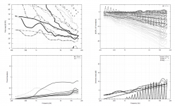
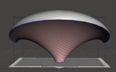
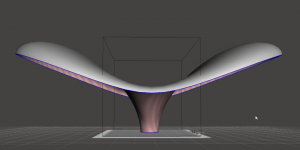
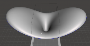
I took some of the R-OSSE designs that Mabat created, and messed around with them, yielding the attached results.

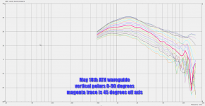
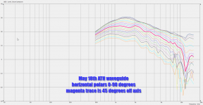
One of the interesting/unexpected results was that horizontal directivity was narrower than vertical directivity, even though the angle of the waveguide is larger. I think that's due to diffraction, basically the horizontal dimension is a small fraction of the vertical dimension.

Because the horizontal dimension is smaller, I think the wavefront is transitioning from a state where it's radiating into 90 degrees, then 180 degrees, then 360 degrees, as frequencies get lower. This has the effect of "shading" the output on the horizontal axis.

 

[Patrick Bateman]

Here's the configuration file:




R-OSSE = {
R = 150 + 100 * abs(sin(p))^2 ; [mm]
r0 = 17 ; [mm]
a0 = 15 ; [deg]
a = 45 ; [deg]
k = 1.6226 + 6*abs(sin(p))^2.1429; []
r = 0.32683 ; []
b = 0.13157 ; []
m = 0.81285 ; []
q = 4.011 ; []
}

Source.Contours = {
zoff -2

point p1 4.68 0 2
point p2 0 14 0.5
point p3 1 15 0.5
point p4 0 16 0.5
point p5 0 17 1
cpoint c1 -18.59 0
cpoint c2 0 15

arc p1 c1 p2 1.0
arc p2 c2 p3 0.75
arc p3 c2 p4 0.25
line p4 p5 0
line p5 WG0 0
}

Mesh.LengthSegments = 36
Mesh.AngularSegments = 48
Mesh.ThroatResolution = 5
Mesh.MouthResolution = 9
Mesh.WallThickness = 8
Mesh.RearResolution = 20

Mesh.SubdomainSlices = 35
Mesh.InterfaceOffset = 25
Mesh.InterfaceDraw = 0

ABEC.MeshFrequency = 1000
ABEC.NumFrequencies = 48
ABEC.Abscissa = 1
ABEC.SimType = 2
ABEC.f1 = 500
ABEC.f2 = 16000

ABEC.Polars:SPL_H = {
MapAngleRange = 0,90,19
}

ABEC.Polars:SPL_H_NORM = {
MapAngleRange = 0,90,19
NormAngle=10
}

ABEC.Polars:SPL_V = {
MapAngleRange = 0,90,19
Inclination = 90
}

Output.ABECProject = 1
Output.STL = 1

Report = {
PolarData = "SPL_H"
NormAngle = 10
MaxAngle = 90
}

 

[mabat]

Yeah, the somewhat narrowed horizontal directivity caught my attention already in the measurements Dkalsi showed. That was ST260-KVAR vs ST260 which are both about the same size (i.e. ~260 mm). That's definitely an interesting outcome -

https://www.diyaudio.com/community/...-design-the-easy-way-ath4.338806/post-7015019

 

[mabat]

Strange flowers

 

[mabat]

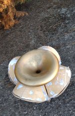
These are the ST260 (brass at the back), 1.4" KVAR (the big one) and its 1:2 scale model in grey.
The ST260 is the old petal construction (quite laborous), the KVAR is assembled from 5 pieces (base + 4 petals, pretty easy) and the small one is made from just two pieces (throat +mouth).

 

[mabat]

Finally working on a full-3D report. In a general case we need to calculate the radiated power properly -
Here's an equally-spaced sampled sphere (100 a 200 points).

 

[TNT]

Would it help to color the dots to understand their position better?