Hello Dave,
Thank you for the access to your tool!
Here is a quick feedback of my installation of PETTaLS.
Our laptops run usually under Linux so I did a quick test with Wine but something was missing. I didn't push further.
So I have restarted a previous laptop under Windows (a Lenovo Yoga 2 I3, windows 8...).
No real issue in the installation. Just the need to download some C++ library (VCRUNTIME140.dll). That done, PETTaLS was installed with an icon on the desktop as I requested.
At 1st launch, I was wondering if it was ok due to the long time to launch the Matlab runtime... but yes, it was ok.
On this laptop (I don't remember the screen resolution), I had to move the taskbar usually at the bottom to the left of the display to get an almost full screen. Almost because the top of the titles of the upper plots are under the matlab window top bar. Not a big issue.
A first simulation up to 2k was done in about 3s (it is not a powerful laptop!).
About the GUI, you could think maybe to add a mark in the plot to remind the simulation was limited in modes.
All the fields are in International Units except the Box Depth... maybe a change? Neither a big issue.
It is very easy to change any field in the GUI.
Probably due to my slow laptop and my first use, I didn't find easy to get information on a point of the FR or the IR. It is much more pleasant in the impedance plot. In fact, I won't be able to say how I got the "delete data tips" menu...
I also tested a simulation up to 20k... about 25mn... I understand the 2k by default. It was about 1s per frequency (mode?). Waiting for the plots update, I was wondering the reason... I ran on this laptop my first DML simulation based on the Finite Difference Method with some large arrays and linear system solving, it was slow also but here I imagine it as to loop on the modes, on the frequency range for each (probably on a log scale?) and on the 2D of the plate to get the velocity. All being based on formulas, under Python it is the job of Numpy to work on arrays (matrix)... sorry this is my developer side who think loud!
For the SPL 80dB scale for the SPL is too large. 50dB is more usual.
In the IR plot, I have a change at about 1500Hz like a scale effect (suddenly, the yellow/green level expend on time).
You will have maybe to think to several time scale for the IR. A 200ms is maybe relevant for a 20Hz frequency but not from a auditory point of view. 50ms is already a long time. When we will look at time EQ for DML, the horizon will be in my opinion much below 10ms.
For further test, I will probably wait for a Linux version...
Of course I point here issues or possible improvements. For the rest : thank you again to share all of that with us.
Christian
Thanks for the great feedback everyone! I've recompiled with a few changes added in, and you should be able to re-download easily from the Google Drive link if you want to:Hi Dave:
Thanks for the release.
I messed around with it and have a few questions :
1/ Materials - I figure the pre-sets just prefill the properties boxes and we can adjust them to suit other materials ? ie - start with anything and change to your desired material properties via the boxes. In that case, to make it clear, why not add a custom material which leaves the boxes blank?.
2/ I ran a few compare cycles and after a couple the comps slowed to a crawl (my desktop is pretty quick) - then I found there was no way to abort a run so I had to ctrl-alt-del - stop matlab process? - Is that correct or did I miss something?
3/ I hope the next release will allow selective mixed support cases.
4/ I really hope the next release will allow anisotropy 🙂
5/ It would be good if comparison graphs changed colours.
No doubt more to come both ways
Thanks again
Eucy
- A stop button to kill execution if the simulation is taking too long.
- On that same note, a field that shows you how many modes you're simulating based on the frequency and panel setup. Once this gets above 1000 modes, the simulation starts to slow down big time.
- The surface velocity appears for each simulated frequency as the simulation runs. It's fun to look at. This slows down the simulation, so I also added a checkbox to turn it off.
- each line in the frequency response comparison is a new color.

Mistakes are always possible 🫣I'm really sorry that I have offended you, I don't think you're a liar or incompetent, but the clip seemed to show so obviously one exciter jumping because of low peak overload, and the other not, that I thought you must have made a mistake with the wiring. That's all. Again my apologies. Hans
But what about my option (c).
When exciters are close, this does not necessarily mean that they are in phase throughout their frequency response.
They can be inphase, out of phase or anywhere in-between these two phases.
This puzzled me at first.
But if you think of the stationery exciter as being inphase with the panel at its position and the other exciter bouncing around out of phase at its position on the panel.
This explains why one is moving and the other is stationery.
The exciter that is bouncing could also be somewhere in-between the two phases, this would cause sideways wobbling, which would look pretty much the same with the naked eye.
These are my thoughts on this subject.
Steve.
Hello Dave,I added a Linux installer to the webpage. I compiled the app on Ubuntu - hopefully it works on your Linux distribution.
There is apparently a bug where dropdown menus don't work unless you add "export ENABLE_QWEBWINDOW=true" before calling the app. This fix worked for me. The app actually seems to run more quickly in Linux!
I have installed the Linux version (laptop DELL I7 with Ubuntu 24.04). It runs fine. I had just some doubt first how to launch the installer to adopt a "sudo ./PETTaLSFree_Linux_web.install" to allow it to install in the default directories proposed (/usr/...).
It seems there is nothing in the installer to add the application in the application menu. This is not a problem. I found the bash script to launch with the path to the Matlab runtime as parameter.
For the next users, a short explanation should help.
Some version number might help also.
I haven't seen really a dropdown menu bug (in the way the dropdown menus worked) but with "export ENABLE_QWEBWINDOW=true" it seems more easy to change the numeric values.
The stop button works... but I don't understand how the highest frequency value works. The surface velocity map is stopped at this value but the Current frequency is increased up 20k before the FR is displayed so the simulation time remains the same. Of course with this laptop is the simulation time is fully acceptable.
It is great to see in the velocity map the modes.
Next step will be to use it for the panels I can test.
Christian
Thanks again Dave, the changes are greatThanks for the great feedback everyone! I've recompiled with a few changes added in, and you should be able to re-download easily from the Google Drive link if you want to:
This is compiled into the Linux version too.
- A stop button to kill execution if the simulation is taking too long.
- On that same note, a field that shows you how many modes you're simulating based on the frequency and panel setup. Once this gets above 1000 modes, the simulation starts to slow down big time.
- The surface velocity appears for each simulated frequency as the simulation runs. It's fun to look at. This slows down the simulation, so I also added a checkbox to turn it off.
- each line in the frequency response comparison is a new color.
A bit more feedback : (what a pandora's box you've opened!!)
1/ On the FR angle response, there's a small circle tailing me around but not near the cursor ??
2/ The dropdowns work on the FR angle graph but the 3d etc don't work on the velocity map and when you pick the 3d button, it won't change back to pan ? (edit - after clicking on the dropdowns in the angle freq graph, I can no longer interrogate it with the mouse - no box appears)
3/ When comparing, a change in the panel size forces the high frequency range to revert to the default 2000 - can this be made to stay as selected until manually changed?
4/ The Q factor is of high importance to practical material selection and it would be good to get some more data on realistic figures for often used materials like plywood (however, the damping will of course be significantly affected/modified by chosen surface treatments - a matter discussed at depth in this forum)
5/ How hard would it be to get an average response over a chosen angle rather than +/- 90?? - It may be more real-world meaningful to limit it to +/- 30 (or 40) or so for example.
6/ Can you add a lower bound frequency box to limit the lowest comp and graph range instead of always starting from 0?
Of interest to me is that juggling aspect ratios seems to yield a best factor of 2.333 rec (7/3) for the smoothest freq response under SSSS conditions.
Thanks again
Eucy
Last edited:
Steve,When exciters are close, this does not necessarily mean that they are in phase throughout their frequency response.
They can be inphase, out of phase or anywhere in-between these two phases.
This puzzled me at first.
But if you think of the stationery exciter as being inphase with the panel at its position and the other exciter bouncing around out of phase at its position on the panel.
The reason this seems unlikely to me is because exciters bounce like that is only when they are driven at very low frequencies, close to their "magnet" fs. At least, that is my experience. For the larger exciters (20W+) that frequency is usually under 50 Hz, though for smaller exciters it's usually a little higher, like maybe 100 Hz.
But at such low frequencies, the modal shapes of the panel typically look something like the first image below. That is, the antinodal areas are quite large. So in order for the two exciters to be at locations that are out of phase with each other, the exciters would have to be pretty far apart. If they are close together, they are either at locations that are in-phase, or are at locations that don't have much displacement, like say on either side of the blue centerline.
At higher frequencies, the modal shapes look more like the second image. At such frequencies the issue you describe is far more likely (inevitable maybe), as the antinodal regions are much smaller. Hence the out of phase regions are much closer, and two closely placed exciters could indeed be at location of different phase. However, such frequencies typically are far above the exciter magnet resonance, so would not be likely to cause an exciter to bounce like that.
My take, anyway.
Eric


Dave,Thanks for the great feedback everyone! I've recompiled with a few changes added in, and you should be able to re-download easily from the Google Drive link if you want to:
Great changes. I haven't downloaded the new version yet, but those sound good.
I'm not sure why, but sometimes it was hanging up and just stopped working, and I would have to restart to run another simulation. And my d*** Norton program has to check it for "suspicious code" every time!
One thing that might be nice would be some indication that it is actually making progress. Like when I ask for a Impedance plot or new velocity map, there can be some delay and I never know if it's actually working on something, or hung up.
Also, the entry fields for properties are rather huge. Maybe space could possibly be used in a better way. I guess maybe it will be in the advanced version.
I hope to play with it more this weekend!
Eric
Eric.
I always find your pictures very pretty, but is that it.
Where is the pistonic (pulse) action and the PIP.
These pictures are too simplistic.
Showing only dml standing waves.
The panel will be flexing in all directions.
You make it sound like the exciter is suffering from magnet resonance, but if in tandem they should be resonating together.
The exciters will be affected differently by the different bends in the panel material in their different locations.
I feel another drawing coming on.
By hand that is.
Steve.
@EarthTonesElectronics
Dave,
Concerning the challenge for the model when the plates are very thin, and the number of modes starts to explode, would it be possible to use "infinite plate mobility theory" to speed up the calculation without too much loss of accuracy? I will readily admit I'm out of my depth here, but I thought I would mention it in case it's useful.
I guess the idea would be to use the modal model at low frequencies, but when the number of activated modes becomes sufficiently high, you would switch to using infinite plate mobility to model the response.
Eric
https://www.hambricacoustics.com/In19_inf_panel.pdf
Easy : switch to Linux. There is a thread in the forum where people share some experiences. Some run even Windons in a Linux machine in a virtual machine. A bit touchy maybe.And my d*** Norton program has to check it for "suspicious code" every time!
Don't you see the "current frequency" changing?One thing that might be nice would be some indication that it is actually making progress.
Windows... I never know what with it what my computer is doing... But don't worry, for sure something important for you!Like when I ask for a Impedance plot or new velocity map, there can be some delay and I never know if it's actually working on something, or hung up.
Christian
What does that mean in words of coincidence frequency? I mean, if the coincidence frequency becomes then very high, it might not be a use case as then the speed of the waves in the plate would be (too?) slow? It happened my panels were too thin, they don't work.Concerning the challenge for the model when the plates are very thin, and the number of modes starts to explode,
Christian
@EarthTonesElectronics
Hello Dave,
One question about your simulator...
Below is a panel, in blue force driven, in pink with a DAEX25.
In my mind, to drive the panel with a force is a bit like driven it with a current source. When it is an exciter it is voltage driven, with a voltage to get the power specified (supposing to use a kind of normalized impedance?)
From that, I expected to see higher resonance peak with a force. In a voltage driven exciter, the back emf gives a better control of the panel.
Am I wrong somewhere? Probably...
Christian
Christian,What does that mean in words of coincidence frequency? I mean, if the coincidence frequency becomes then very high, it might not be a use case as then the speed of the waves in the plate would be (too?) slow? It happened my panels were too thin, they don't work.
Christian
Sorry, I'm not certain what you are asking, or even if you are asking me, or more likely Dave?
What I was referring to was the fact that if the plate is very thin (or even very low modulus, or very high density, or some combination) then the number of modes between 20 Hz and 20 kHz is much larger than for a thicker plate. Since the model presumably works by summing the contributions of all the modes, it may run very slowly when there are so many modes with contributions to add up. So my question had only to do with the way the model operates on such a panel, not regarding what the actual performance of that panel would be.
But I too have wondered if the panel can be too thin. For example, what happens when the panel is so thin that the panel wave speed at even 20 kHz is far below the speed of sound in air? I suspect (as I assume you are also thinking), that the radiation efficiency would be poor in that case. But is that correct?
Eric
Yes, for sure, I've already got this on my list of things to work on eventually (but time is finite, unfortunately). Large sandwich plates would take way too long to simulate without crossing over to a non-modal set of equations at some point.@EarthTonesElectronics
Dave,
Concerning the challenge for the model when the plates are very thin, and the number of modes starts to explode, would it be possible to use "infinite plate mobility theory" to speed up the calculation without too much loss of accuracy? I will readily admit I'm out of my depth here, but I thought I would mention it in case it's useful.
I guess the idea would be to use the modal model at low frequencies, but when the number of activated modes becomes sufficiently high, you would switch to using infinite plate mobility to model the response.
Eric
https://www.hambricacoustics.com/In19_inf_panel.pdf
Good point - the "point force" nowadays is more of a "point" than a "force." It's got the same electrical model as the exciters, but just without any resonance and without any coupling shape. It'll be interesting to add the pure force (or current source) in and see how it compares.@EarthTonesElectronics
Hello Dave,
One question about your simulator...
Below is a panel, in blue force driven, in pink with a DAEX25.
In my mind, to drive the panel with a force is a bit like driven it with a current source. When it is an exciter it is voltage driven, with a voltage to get the power specified (supposing to use a kind of normalized impedance?)
From that, I expected to see higher resonance peak with a force. In a voltage driven exciter, the back emf gives a better control of the panel.
Am I wrong somewhere? Probably...
Christian
View attachment 1428389
@EarthTonesElectronics
Hello Dave
A couple of further suggestions
1/ For the surface velocity map - replacing the frequency box with a slider would be way more user friendly
2/ Related to the above - move the Current Frequency box from below the Run/Stop to below the Surface Velocity Map so the map frequencies can be followed during a run without constantly glancing down at the frequency box
Regards
Eucy
Last edited:
Hello Dave,Good point - the "point force" nowadays is more of a "point" than a "force." It's got the same electrical model as the exciters, but just without any resonance and without any coupling shape. It'll be interesting to add the pure force (or current source) in and see how it compares.
Clear. I understand it is a king of "ideal point force exciter". So it supposes you have chosen an electrical resistance and a force factor for it? No inductance?
The question was for you and/or David.Christian,
Sorry, I'm not certain what you are asking, or even if you are asking me, or more likely Dave?
What I was referring to was the fact that if the plate is very thin (or even very low modulus, or very high density, or some combination) then the number of modes between 20 Hz and 20 kHz is much larger than for a thicker plate. Since the model presumably works by summing the contributions of all the modes, it may run very slowly when there are so many modes with contributions to add up. So my question had only to do with the way the model operates on such a panel, not regarding what the actual performance of that panel would be.
But I too have wondered if the panel can be too thin. For example, what happens when the panel is so thin that the panel wave speed at even 20 kHz is far below the speed of sound in air? I suspect (as I assume you are also thinking), that the radiation efficiency would be poor in that case. But is that correct?
Eric
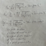
I see your point.
From my paper about panel materials, I see : A.f0.fc = c²
fo being the first mode
fc the coincidence frequency
c the speed of sound in the air
A is more or less the panel area depending on the edge conditions
The thickness is somehow resulting or let say the parameter to adjust fc and A the parameter to adjust f0..and the simulation time will follow.
Thanks Steve.I always find your pictures very pretty
The bouncing of the exciter is a resonance effect that takes at least a few cycles to build up, so any transient is irrelevant to this effect, I feel certain.Where is the pistonic (pulse) action and the PIP.
These pictures are too simplistic.
Showing only dml standing waves.
For all practical purposes, the only direction that the panel deflects is perpendicular to the plane of the surface. Deflections of the panel in any other direction are smaller by orders of magnitude.The panel will be flexing in all directions.
I'm not sure what you thought I meant by "magnet resonance". But what I was calling "magnet resonance" is what Xcite refers to as "Fs Magnet" in their specs. That refers to is the frequency at which there is a peak in the impedance measurement (when the impedance test is performed by attaching the exciter foot to a rigid body without constraining the magnet). In the curve at the bottom, I circled in red the peak at 40.5 Hz corresponding to the Fs-Magnet of that exciter. Fs-magnet for any exciter reflects the frequency at which the exciter tends to really bounce, and corresponds essentially to the resonance frequency of the magnet mass combined with the spring constant of the spider. In fact, it is the bouncing of the exciter at this resonance which causes the spike in the impedance curve, by creating "back EMF".You make it sound like the exciter is suffering from magnet resonance,
I do think that the properties of the panel itself can slightly shift the frequency at which an exciter will bounce, but other than that, it is not the panel's motion that causes the exciter to bounce. What makes an exciter bounce is simply driving it at a frequency close to its Fs-Magnet.
I'm looking forward to it.I feel another drawing coming on.
By hand that is.
Eric
Dave,This is very cool. I think you should present this at an acoustics conference, but maybe that's more my thing than anybody else's in this forum!
I think I share the same general concern as Christian - I see how the thickness of the plate is normalized out because it's included in the "thin plate index," but is the beam length also unimportant in the results shown in that graph?
I can't believe I missed this until now. Thanks for your comment. If you present it we can be co-authors! I did think was pretty interesting myself that the non-dimensional "thin plate index" value turned out to be independent of thickness (t). Before doing the math I was assuming there would still be t or t^2 or t^(1/2) left over on the right side. But there isn't and "index" depends only on E, rho, and nu, but not t (or L).
Regarding your question about beam length, I'm not sure I understand your question fully. And you may not even remember it yourself by now! But I think the answer is that the beam length is not important.
In the FEA model, I could have made the beam 2.5 times longer, but the frequency corresponding to a given wavelength would have been the same. But using simple supports was critical to being able to do this analysis, because simple supports are exactly like nodes, that is, they have zero displacement and zero bending moment. I still fear this isn't exactly the answer to your question.
Eric

Attachments
Dave,Thanks for the great feedback everyone! I've recompiled with a few changes added in, and you should be able to re-download easily from the Google Drive link if you want to:
- A stop button to kill execution if the simulation is taking too long.
- On that same note, a field that shows you how many modes you're simulating based on the frequency and panel setup. Once this gets above 1000 modes, the simulation starts to slow down big time.
- The surface velocity appears for each simulated frequency as the simulation runs. It's fun to look at. This slows down the simulation, so I also added a checkbox to turn it off.
- each line in the frequency response comparison is a new color.
I finally had time today to load the new version and I'm having great fun with it. I really do love the "real time" surface velocity map. It is mesmerizing to watch and so far I don't mind that it takes longer to run! It would be nice if the frequency "counter" was closer to the velocity map, like above or below it, or even overlaid on top, so you could more easily see what is happening at each frequency.
I have the same comment as Eucy about the frequency limit setting. It's annoying when you set it to a value and then it reverts back to 2000 Hz. Once you change it during a session I think it should stay fixed until you change it again manually.
It's running more reliably for me than the earlier version too it seems. But sometimes there are still odd delays, like when I request an impedance plot. Sometimes it comes up immediately, and other times it takes like 20 seconds. There is also sometimes a delayed reaction to the run command as well by 10 or 20 seconds, and other times it starts immediately. A few times I ended up pressing "run" a second time because it seemed like nothing was happening, then pressed the "stop" (for some reason), and then saw it immediately start up again, as if it was actually running twice simultaneously because I had hit "run" twice.
I'm not sure what we should expect to be able to do with the graphs that show up on the "normal" screen. With the "auxiliary" plots like the impedance plot, the zoom and pan etc functions seem to work mostly, but they never work for me on the SPL plots.
I do wonder if some of my issues are more related to my crappy old computer than to your software.
Eric
Eucy,2/ The dropdowns work on the FR angle graph but the 3d etc don't work on the velocity map and when you pick the 3d button, it won't change back to pan ? (edit - after clicking on the dropdowns in the angle freq graph, I can no longer interrogate it with the mouse - no box appears)
What is the "3d" you are talking about? I don't know if it works for me because I don't know what it is!
I agree it would be nice to have realistic Q factors for materials built into Dave's the model. But I'm not sure it's a huge hurdle if we don't. I say that because the height and sharpness of the peaks in the impedance curve are extremely sensitive to Q factor. So the key for us modelers is to have an impedance rig of our own. Then we can get a pretty good idea of the Q of any particular material my comparing an actual measured impedance curve to the result of Dave's model, and just iterate the model with different values of Q until the height and sharpness of the impedance peaks are similar in the model and measurement. I don't think it's too critical to be "exact" with the Q value, you just need to be in the ballpark I think. As Dave has noted previously, Q isn't really even a constant for real materials, so there is no exact value anyway.4/ The Q factor is of high importance to practical material selection and it would be good to get some more data on realistic figures for often used materials like plywood (however, the damping will of course be significantly affected/modified by chosen surface treatments - a matter discussed at depth in this forum)
This does mean we need at least a sample panel of the material in question, and REW with an impedance rig, however.
Eric
- Home
- Loudspeakers
- Full Range
- A Study of DMLs as a Full Range Speaker