300Hz-1.5kHz attached.Have you tried the Field view in the vertical plane to see what is happening?
Attachments

I took the A460G2, basically cut it at the apex and tried a baffle-mounted version. It's not that bad after all -
It's ⌀356 x 160 mm. Simulated with the 36-STD-1 adapter (apparently, the sim starts to fail numerically around 12 kHz):


So, this is also an option. I can try also a rectangular version, but this is actually pretty good already, I expected it to be a bit worse, honestly.
Maybe I'll only scale it down a bit so that it fits 350x350mm bed in one piece 🙂
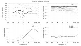
Polars on the diagonal (@2m, 0 - 180 / 5°):

It's ⌀356 x 160 mm. Simulated with the 36-STD-1 adapter (apparently, the sim starts to fail numerically around 12 kHz):
So, this is also an option. I can try also a rectangular version, but this is actually pretty good already, I expected it to be a bit worse, honestly.
Maybe I'll only scale it down a bit so that it fits 350x350mm bed in one piece 🙂
Polars on the diagonal (@2m, 0 - 180 / 5°):
Last edited:
You know what? The round version is actually better than a square (I tried a few different) -


Some would say it's not surprising, but I do find it a bit surprising 🙂
Some would say it's not surprising, but I do find it a bit surprising 🙂
Hi,
New to ATH but very impressed with all the capabilities 🙂
Simulated some OSSE Waveguides without any problems. Now wanting to do a free standing asymetric R-OSSE Waveguide and encountered some difficulties.
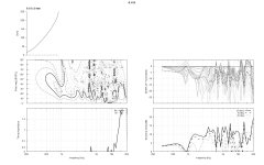
I first started with the same Resolution settings as my successful OSSE trials (4mm throat, 10mm Mouth, 10mm rear wall, 1000Hz Mesh frequency) and got absolute chaos as results. Seeing that other people used Mesh frequency only and no resolution I upped that to 10,000hz (as 20000Hz had over 10k mesh elements), still no correct results. (see first image)
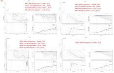
Made some trials on a smaller horn and it seems like anything under 20kHz Mesh frequency gives weird results. (see second image)
No feeling a bit lost on how to continue. Are there any ways to reduce the resolution while not giving completly false results? Why is resolution so diffrent with R-OSSE than OSSE?
Here is my script if you can spot any issues:
New to ATH but very impressed with all the capabilities 🙂
Simulated some OSSE Waveguides without any problems. Now wanting to do a free standing asymetric R-OSSE Waveguide and encountered some difficulties.
I first started with the same Resolution settings as my successful OSSE trials (4mm throat, 10mm Mouth, 10mm rear wall, 1000Hz Mesh frequency) and got absolute chaos as results. Seeing that other people used Mesh frequency only and no resolution I upped that to 10,000hz (as 20000Hz had over 10k mesh elements), still no correct results. (see first image)
Made some trials on a smaller horn and it seems like anything under 20kHz Mesh frequency gives weird results. (see second image)
No feeling a bit lost on how to continue. Are there any ways to reduce the resolution while not giving completly false results? Why is resolution so diffrent with R-OSSE than OSSE?
Here is my script if you can spot any issues:
Code:
R-OSSE = {
  R = 300*200/sqrt((300*sin(p))^2+(200*cos(p))^2)
  a = 45*30/sqrt((45*sin(p))^2+(30*cos(p))^2)
  r0 = 17.78
  a0 = 0.5
  k = 2
  r = 0.2
  m = 0.85
  b = 0.2
  q = 5
}

Mesh.AngularSegments = 64
Mesh.LengthSegments = 20
Mesh.SubdomainSlices =
Mesh.Quadrants = 1
Mesh.RearShape = 1
Mesh.WallThickness = 10.0 ; [mm]
Source.Shape = 1

Output.STL = 1
Output.ABECProject = 1

ABEC.SimType = 2 ; 1 = infinite baffle
ABEC.f1 = 300 ; [Hz]
ABEC.f2 = 20000 ; [Hz]
ABEC.NumFrequencies = 60
ABEC.MeshFrequency = 10000 ; [Hz]

ABEC.Polars:SPL_H = {
MapAngleRange = 0,90,19 ; first angle, last angle, number of points
NormAngle = 10 ; normalization angle [deg]
Distance = 3 ; [m]
Offset = 235 ; [mm]
}

ABEC.Polars:SPL_V = { ; diagonal polars
MapAngleRange = 0,90,19 ; first angle, last angle, number of points
NormAngle = 10 ; normalization angle [deg]
Distance = 3 ; [m]
Offset = 235 ; [mm]
Inclination = 90 ; [deg]
}

Report = {
Title = "4.4 H"
PolarData = SPL_V
NormAngle = 0
Width = 1600
Height = 1000
GnuplotCode = 3x2n.gpl
}
Attachments
That has done the trick on the small horn 🙂 (see image)
Makes sense, issue was probably triggered by the backside of the mouth rollback, thanks for the tip. "NUC (Non-Uniqueness Compensation) fails if boundaries are opposite and very close. In this case switch off NUC at menu Global/BEM Parameters."
Makes sense, issue was probably triggered by the backside of the mouth rollback, thanks for the tip. "NUC (Non-Uniqueness Compensation) fails if boundaries are opposite and very close. In this case switch off NUC at menu Global/BEM Parameters."
Attachments

I performed a quick benchmark BEMPP vs ABEC3 using the loudspeaker form BEMPP loudspeaker tutorial. I modified original GMSH geo file to increase the mesh density
The both benchmarks were run for single 1000Hz frequency. It seems that BEMPP uses much more faster solver (iterative GMRES) than ABEC3. It took ~15.5 s to solve the problem on my 14 cores workstation in BEMPP. Whereas ABEC3 spent approximately 1127s to solve the same problem. It should be noted, that ABEC3 use single core to solve single frequency, whereas BEMPP use all cores. For an ideally parallelizable problem, the BEMM should be faster only by a factor of 14 because my workstation has 14 cores. However BEMPP is actually faster by a factor of 73 ! Which suggests that BEMPP uses a much more efficient solver.
I'll try to figure out BEMPP settings to run the same benchmark on a single core for a solver efficiency comparison vs. ABEC3.
May I ask which version of bempp you used (bempp [C++], bempp-cl [python + opencl/numba] or bempp-rs [rust])?
I have started playing with bempp-cl which seems to the current version and it is not running efficiently for me. It does have periods running with a full set of threads but much of the time it is running single threaded. With your benchmark it is took about 50 seconds to assemble and 325 seconds to solve. In contrast a simple threaded "teaching" C BEM code took 7 seconds to assemble and 6 seconds to solve using a direct method. This is in line with your bempp results and what I was expecting to see for bempp.
Did you continue looking at bempp?
Maybe this is due to circle-in-a-square version having more diverse pathlengths from source to baffle edges and backside edges, spreads the diffraction?You know what? The round version is actually better than a square (I tried a few different) -
View attachment 1445147 View attachment 1445148
View attachment 1445149 View attachment 1445150
Some would say it's not surprising, but I do find it a bit surprising 🙂
what's the diagonal look like?Some would say it's not surprising, but I do find it a bit surprising 🙂
- If anyone wants to improve the polar map presentation in the default report, update the highlighted lines in the file '.../bin/lib/scripts/2x2n.gpl':
# Polar Map
set contour base
set view map
unset surface
set style textbox noborder opaque
set cntrparam level discrete 6,3,2,1,-1,-2,-3,-4,-5,-6,-9,-12,-15
set cntrlabel start -1 interval -1 font "Arial,11"
set grid xtics mxtics ytics
set xtics add ("200" 200, "500" 500, "1k" 1000, "5k" 5000, "10k" 10000, "" 15000, "20k" 20000)
set logscale x
set format y "%.0f°"
set xrange [200:20000]
set yrange [0:R_MAX_ANGLE]
set ylabel "Polar map [dB SPL]" offset -2,0
splot "pmap.txt" u 2:1:3 w l lw 1 not, \
"" u 2:1:3 w labels boxed not
View attachment 1124525
My enhancements aren't as nice as this, but I created a modified version of "2x2n.gpl" that's located under the "scripts" directory in your ATH folder.
All of my monitors are 4K, and my enhancements simply make the fonts larger and the lines thicker, so that reports at high resolution look better. I also changed the scale, because I rarely run sims above 16K or below 250Hz.
If you use a resolution of 1920x1080 or less in the "report" stanza of your config file, the fonts will probably be too big, but if you're using high resolutions, it's handy.
I've attached two sims, one with the "fat lines" and one with the stock config.
Below is the config, if you want to use it, just replace the contents of 2x2n.gpl , or create a new gpl file and reference it in your reports stanza, as described by Mabat in his post above.
load 'static.txt'
load 'param.txt'
set terminal pngcairo monochrome size R_W,R_H font "Verdana,27"
set output R_FILE.'.png'
set multiplot layout 2,2 \
margins 0.1,0.96,0.1,0.92 \
spacing 0.1,0.06 \
title R_TITLE font "Verdana,26" noenhanced
# Polar Map
set contour base
set view map
unset surface
set style textbox noborder opaque
set cntrparam level discrete 1,-1,-3,-6,-10,-20
set cntrlabel start -3 interval -1 font "Courier New,33"
set grid xtics mxtics ytics
set xtics add ("250" 250, "500" 500, "1k" 1000, "2k" 2000, "4k" 4000, "" 8000, "16k" 16000)
set logscale x
set format y "%.0f°"
set xrange [250:16000]
set yrange [0:R_MAX_ANGLE]
set ylabel "Polar map [dB SPL]" offset -2,0
splot "pmap.txt" u 2:1:3 w l lw 4 not, \
"" u 2:1:3 w labels boxed not
# normalized SPL curves + Sound Power
set grid xtics mxtics ytics
unset colorbox
set yrange [-25:5]
#set ytics ("0" 0,"-5" -5,"-10" -10,"-15" -15,"-20" -20,"-25" -25,"-30" -30)
set ytics ("0" 0,"-5" -5,"-10" -10,"-15" -15,"-20" -20)
set ylabel "dB SPL (".R_NORM_ANGLE."° normalized)" offset 0,0
unset format y
plot "polars_norm.txt" u 1:2:3 not w l lw 4 palette, \
"spower_norm.txt" u 1:2 w l dt "-" lc rgb "black" lw 4 t "SP"
# Throat Impedance
set yrange [0:2]
set ytics ("0" 0, "0.2" 0.2, "0.5" 0.5, "1" 1, "1.5" 1.5)
set xlabel "Frequency [Hz]"
set ylabel "Throat Impedance"
plot "radimp.txt" u 1:2 w l lw 4 lc rgb "black" t "Re", "" u 1:3 w l lw 2 t "Im"
# DI, etc.
set yrange [0:25]
set ytics ("0" 0, "5" 5, "10" 10, "15" 15, "20" 20)
set xlabel "Frequency [Hz]"
set ylabel "Directivity Index [dB]" offset -1,0
plot "DI.txt" u 1:2 w l lw 4 t "on-axis", \
"" u 1:3 w l lw 4 t "10 deg", \
"" u 1:4 w l lw 4 t "20 deg"
unset multiplot
Attachments
A couple of pic's for the evening:

 My first A460 is assembled. It was printed in white Overture Turbo PLA. I used the 2 piece adapter, with the throat piece printed in gold silk PLA (with a tip of the hat to a previous poster who showed a gold throat in a black horn). No filler or paint, and won't be for at least some time to come. The woofer is the FaitalPro 15FH500 (from when Madisound blew out a batch of them for 1/2 price), in a cheap plywood box that was re-used from an old project and happened to be a good size. Better looking woofer cabinets will happen before any cosmetic work on the horns, and it will be a while before I can get to those.
I'm pretty happy with how my brackets turned out. They seem plenty strong, and are stable enough to stand up without being bolted down. They are a nice snug fit on the adapters, the set screws are barely snugged up so nothing can buzz. the setscrews are 33 mm long so they have plenty of engagement in the relatively tiny threads tapped into the plastic. If the threads ever fail I'll have to try using some heat set threaded inserts.
The second petal ring is glued up and curing overnight.
I'd show a FR sweep, but it looks just like every other FR for this driver combination. Very smooth!
Bill
That's fascinating to observe. I've never encountered this in a real situation but apparently it can happen (and it's actually rather surprising that it doesn't happen every time).300Hz-1.5kHz attached.
Guess I'm just unlucky 🙂I've never encountered this in a real situation
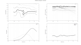
Just to further illustrate the effect, here's what the system directivity would look like if the waveguide didn't interfere with the woofer's vertical pattern:


Maybe it happens more often that I (we) would think. The truth is that I was many times surprised by the rather large and not really anticipated DI step in this area, in reported measurements by others. It's definitely worth investigating further. Maybe it would benefit from designing the waveguides a bit differently then...
Shallow and freestanding with proper c-c spacing to make smooth DI and power 😉 Fact is, on a multiway speaker structure of one transducer is in immediate acoustic environment of the other, and some disturbance to the field happens no matter what. One could go coaxial for bit different looking graphs, but that has similar issues, woofer is not ideal waveguide for tweeter or tweeter waveguide masks the woofer and so on, and it's inevitable.
Most of the time this stuff is hidden with such big speakers, because it needs > 6ms windowing in measurements to get enough resolution to see these, cannot get that measuring inside a domestic room.
Most of the time this stuff is hidden with such big speakers, because it needs > 6ms windowing in measurements to get enough resolution to see these, cannot get that measuring inside a domestic room.
Last edited:
Yeah, those were my thoughts as well, this may have some truth to it.Most of the time this stuff is hidden with such big speakers, because it needs > 6ms windowing to get enough resolution, cannot get that measuring inside a domestic room.
Another approach is really to extend the bandwidth of a (big) horn as low as possible.
Separating the two sources physically at least a bit apart (completely, i.e with a gap between) may also help, it seems. That would need to be investigated.
JBL M2 shows a similar dip in the published measurements, BTW, which should be all high-quality acoustic data.
Last edited:
- Home
- Loudspeakers
- Multi-Way
- Acoustic Horn Design – The Easy Way (Ath4)