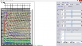
Here is GK-71 pentode model:
Code:
**** GK_71 ******************************************
* Created on 11/15/2022 00:27 using paint_kip.jar
* www.dmitrynizh.com/tubeparams_image.htm
* Plate Curves image file: gk-71.png
* Data source link: <plate curves URL>
*----------------------------------------------------------------------------------
.SUBCKT GK_71 P G2 G K ; LTSpice tetrode.asy pinout
* .SUBCKT GK_71 P G K G2 ; Koren Pentode Pspice pinout
+ PARAMS: MU=5.136 KG1=9154.28 KP=113.52 KVB=22.49 VCT=25.69 EX=1.492 KG2=22042.68 KNEE=34.18 KVC=1.957
+ KLAM=6.25E-9 KLAMG=3.562E-7 KNEE2=0.95 KNEX=30  KNK=-0.044 KNG=0.006 KNPL=0.1562 KNSL=7.48 KNPR=13.8 KNSR=29
+ CCG=22P CGP=0.15P CCP=24P VGOFF=0.33 IGA=0.004044 IGB=0.384 IGC=30.4 IGEX=1.84
* Vp_MAX=1600 Ip_MAX=950 Vg_step=20 Vg_start=100 Vg_count=20
* X_MIN=62 Y_MIN=165 X_SIZE=422 Y_SIZE=493 FSZ_X=1296 FSZ_Y=736 XYGrid=false
* Rp=1400 Vg_ac=20 P_max=125 Vg_qui=-90 Vp_qui=300
* showLoadLine=n showIp=y isDHP=n isPP=n isAsymPP=n isUL=n showDissipLimit=y
* showIg1=y isInputSnapped=y addLocalNFB=n
* XYProjections=n harmonicPlot=y dissipPlot=n
* UL=0.43 EG2=400 gridLevel2=y addKink=y isTanhKnee=y advSigmoid=n
*----------------------------------------------------------------------------------
RE1  7 0  1G    ; DUMMY SO NODE 7 HAS 2 CONNECTIONS
E1   7 0  VALUE=  ; E1 BREAKS UP LONG EQUATION FOR G1.
+{V(G2,K)/KP*LOG(1+EXP((1/MU+(VCT+V(G,K))/SQRT(KVB+V(G2,K)*V(G2,K)))*KP))}
RE2  6 0  1G    ; DUMMY SO NODE 6 HAS 2 CONNECTIONS
E2  6 0  VALUE={(PWR(V(7),EX)+PWRS(V(7),EX))} ; Kg1 times KIT current
RE21 21 0 1
E21  21 0 VALUE={V(6)/KG1*ATAN((V(P,K)+KNEX)/KNEE)*TANH(V(P,K)/KNEE2)} ; Ip with knee but no slope and no kink
RE22 22 0 1 ; E22: kink curr deviation for plate
E22  22 0 VALUE={V(21)*LIMIT(KNK-V(G,K)*KNG,0,0.3)*(-ATAN((V(P,K)-KNPL)/KNSL)+ATAN((V(P,K)-KNPR)/KNSR))}
G1   P  K  VALUE={V(21)*(1+KLAMG*V(P,K))+KLAM*V(P,K) + V(22)}
* Alexander Gurskii screen current, see audioXpress 2/2011, with slope and kink added
RE43 43 K 1G ; Dummy
E43  43 G2 VALUE={0} ; Dummy
G2   43 K  VALUE={V(6)/KG2*(KVC-ATAN((V(P,K)+KNEX)/KNEE)*TANH(V(P,K)/KNEE2))/(1+KLAMG*V(P,K))-V(22)}
RCP  P K  1G     ; FOR CONVERGENCE
C1   K G  {CCG}  ; CATHODE-GRID 1
C2   G P  {CGP}  ; GRID 1-PLATE
C3   K P  {CCP}  ; CATHODE-PLATE
RE23 G 0 1G
GG G K VALUE={(IGA+IGB/(IGC+V(P,K)))*(MU/KG1)*
+(PWR(V(G,K)-VGOFF,IGEX)+PWRS(V(G,K)-VGOFF,IGEX))}
.ENDS
*$
Attachments
Consolidating two questions I didn't realize I messed up.
What kind of .asc circuit does one use to generate tube curves in LTspice if a known-good model is available?
EL81 has been used as PP pentodes in Philips PA amplifiers long ago.
Philips BX998A table radio used PL81's as direct-coupled series triodes in the bass amp and EL84 for the treble amp. I think this radio used high impedance voice coil speakers (700-800 ohms?)
One Philips datasheet I have to keep re-finding has a small set of as-triode data ( ra=1k, mu = 5.5, gm = 0.0055 @ 250 V, 40 mA, -38V on g1), but no triode curves. It has a 8W plate but with g3 connected to k, & g2 connected to a, they use 10 W as combined plate + screen dissipation).
I have done some LTspice simulation of preamps, but never attempted creating tube curves. Attempting to replicate pentode-as-triode curves for one that has already been done would be a good way to validate one's own plots.
But I am not sure what kind of circuit would do this.
Reading some of the 'Getting Started' web pages is helpful, but one eventually encounters advice to not use certain models.
So obviously not a task to undertake alone (in a vacuum)!
I have a library file for PL81 that Derk Reefman created, as both pentode and triode.
Any recommendations for a 'curve tracer' circuit to pursue this? I don't have an amplifier circuit to simulate. I want triode curves to draw a load line on first.
Thank you
Murray
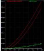
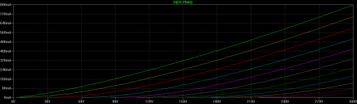
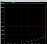
Try the attached LTspice file. It includes the Reefman PL81 pentode model, and the simulation's plot parameters are consistent with the attached Philips PL81 datasheet (bottom of page 4). After running the simulation, place the current probe on the tube's anode to plot the anode current and you should get the plot shown in the attached image.
Attachments

And here are PL81 triode curves. Change the stepping parameters and manual limits to your liking.
Attachments
Last edited:
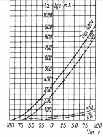
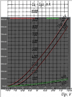
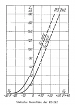
Hi i try to derive some spice model for RS242 DH triode. The model is based on tiny and insuficient informations. At least I didnt find more informations than original TFK sheet. 🙁
a) First I multipied the 2 curves from graph
b) get the data points from Graph Click.
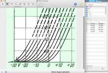
c) Set the Matlab file RS242.m to input in the Norman K. Tuparam Matlab, to fet the Anode chrs in more desirable form.
d) With these anode chrs I checked with Model Paint tools soft for the composite DHT model.
a) First I multipied the 2 curves from graph
b) get the data points from Graph Click.
c) Set the Matlab file RS242.m to input in the Norman K. Tuparam Matlab, to fet the Anode chrs in more desirable form.
d) With these anode chrs I checked with Model Paint tools soft for the composite DHT model.
Code:
****  Composite RS242 DHT *****************************************
* Created on 01/10/2023 22:42 using paint_kit.jar 3.1
* www.dmitrynizh.com/tubeparams_image.htm
*
* Data source link: Telefunken RS242 datas
* Vhaeat = 3.8 [V]
* Iheat    =  0.72 [A]
* Pa-max = 12[W]
* Ia-max = 70[mA]
* Ua-max = 400[V]
*-------------------------------------------------------------------
.SUBCKT RS242_DHT 1 2 3 4 ; P G K1 K2
+ PARAMS:
+ CCG=4.2P
+ CGP=7.7P
+ CCP=3.7P
+ RFIL=5.278
+ MU=17
+ KG1=1950
+ KP=140
+ KVB=250
+ VCT=0
+ EX=1.4
+ RGI=2000
RFIL_LEFT    3  31 {RFIL/4}
RFIL_RIGHT   4  41 {RFIL/4}
RFIL_MIDDLE1 31 34 {RFIL/4}
RFIL_MIDDLE2 34 41 {RFIL/4}
E11 32 0  VALUE={V(1,31)/KP*LOG(1+EXP(KP*(1/MU+V(2,31)/SQRT(KVB+V(1,31)*V(1,31)))))}
E12 42 0  VALUE={V(1,41)/KP*LOG(1+EXP(KP*(1/MU+V(2,41)/SQRT(KVB+V(1,41)*V(1,41)))))}
RE11 32 0 1G
RE12 42 0 1G
G11 1 31 VALUE={(PWR(V(32),EX)+PWRS(V(32),EX))/(2*KG1)}
G12 1 41 VALUE={(PWR(V(42),EX)+PWRS(V(42),EX))/(2*KG1)}
RCP1 1 34 1G
C1 2 34 {CCG} ; CATHODE-GRID
C2 2 1 {CGP} ; GRID=PLATE
C3 1 34 {CCP} ; CATHODE-PLATE
D3 5 3 DX ; FOR GRID CURRENT
D4 6 4 DX ; FOR GRID CURRENT
RG1 2 5 {2*RGI} ; FOR GRID CURRENT
RG2 2 6 {2*RGI} ; FOR GRID CURRENT
.MODEL DX D(IS=1N RS=1 CJO=10PF TT=1N)
.ENDS
*$
Attachments

Last edited:
Ray-Try the attached LTspice file. It includes the Reefman PL81 pentode model, and the simulation's plot parameters are consistent with the attached Philips PL81 datasheet (bottom of page 4). After running the simulation, place the current probe on the tube's anode to plot the anode current and you should get the plot shown in the attached image.
Maybe I am being too literal, but after plotting the pentode sim voltages, and then not matching, I noted you said current probe, and my observation with the 'cursor' probe is that its default is voltage, and the resultant X-Y plots are (uninteresting) V-V lines 😡)
Do I need to figure out how to change the setup for probe/plot to current, or add directives for I(x)?
If directives would each (x) be the sources VP, VCG, VSG, or I(N003) etc.?
Meanwhile, I'll try things & see what happens.
Thank you
Ah, just found right click, Add Traces, and the currents of interest are there.
One hand in my pocket...
I probably could have described this better. After running the simulation, you can move the cursor and left-click on various nodes to plot their attributes. If you hover the cursor over the wire leading from the plate, the cursor turns into a probe symbol and left-clicking on the wire with the probe symbol displayed will plot the voltage on the wire (node). But if you move the cursor over the plate in the tube symbol the cursor shape turns into a clamp-on ammeter symbol. Left-clicking while the ammeter cursor is displayed will plot the current into that node. That is how I displayed the plot attached to my post. You really don't need to use "add trace" in this situation although you certainly can if you want to. There is usually more than one way to accomplish something. 🙂
I hope this helps.
I hope this helps.
That was not supposed to be a mad face I posted...it was auto-corrected to an emoji or similar. Or shape-shifted.Yes, helpful.
Thank you
Now I'll move on to figuring out how Dimitrynizh paints his masterpiece curves. From stick-figures to landscapes will take some practice.
I thought the triode curves looked pretty nice, then realized they've melted by the time they reach the really linear parts!
I rescaled & printed a smaller range to achieve my paper goals. Still very pleasing, and good for something as a triode...TBD what.
... and here it is, the freshly baked 6N6P model! 😀
Based on the most representative triode out of 4 tubes, all burnt-in for 100 hours.
next tube will be the 6N15P, but it will take a bit more time as I have first to buy some 7pin sockets for the burnin.
cheers, Adrian
Code:*6N6P LTspice model based on the generic triode model from Adrian Immler, version i4 *A version log is at the end of this file *100h BurnIn of 4 Novosibirsk factory tubes, sample selection and measurements done in Febr. 2021 *Params fitted to the measured values by Adrian Immler, Febr. 2021 *The high fit quality is presented at adrianimmler.simplesite.com *History's best of tube decribing art (plus some new ideas) is merged to this new approach. *@ neg. Vg, Ia accuracy is similar to Koren models. *@ small neg. Vg, the "Anlauf" current is considered. *@ pos. Vg, Ig and Ia accuracy is on a unrivaled level. *This offers new simulation possibilities like bias point setting with MOhm grid resistor, *Audion radio circuits, low voltage amps, guitar distortion stages or pulsed stages. * anode (plate) * | grid * | | cathode * | | | .subckt 6N6P.i4 A G K + params: *Parameters for the space charge current @ Vg <= 0 + mu = 20.3 ;Determines the voltage gain @ constant Ia + rad = 1k1 ;Differential anode resistance, set @ Iad and Vg=0V + Vct = -0.85;Offsets the Ia-traces on the Va axis. Electrode material's contact potential + kp = 90 ;Mimics the island effect + xs = 1.60 ;Determines the curve of the Ia traces. Typically between 1.2 and 1.8 * *Parameters for assigning the space charge current to Ia and Ig @ Vg > 0 + kB = 0.4 ;Describes how fast Ia drops to zero when Va approaches zero. + radl = 10 ;Differential resistance for the Ia emission limit @ very small Va and Vg > 0 + tsh = 5 ;Ia transmission sharpness from 1th to 2nd Ia area. Keep between 3 and 20. Start with 20. + xl = 1.2 ;Exponent for the emission limit * *Parameters of the grid-cathode vacuum diode + kvdg = 27 ;virtual vacuumdiode. Causes an Ia reduction @ Ig > 0. + kg = 590 ;Inverse scaling factor for the Va independent part of Ig (caution - interacts with xg!) + Vctg = -0.75;Offsets the log Ig-traces on the Vg axis. Electrode material's contact potential + xg = 1.4 ;Determines the curve of the Ig slope versus (positive) Vg and Va >> 0 + VT = 0.11 ;Log(Ig) slope @ Vg<0. VT=k/q*Tk (cathodes absolute temp, typically 1150K) + kVT=0.1 ;Va dependant koeff. of VT + Vft2 = 0.0 gft2 = 20 ;finetunes the gridcurrent @ low Va and Vg near zero * *Parameters for the caps + cag = 3p5 ;From datasheet + cak = 1p85 ;From datasheet + cgk = 4p4 ;From datasheet * *special purpose parameters + os = 1 ;Overall scaling factor, if a user wishes to simulate manufacturing tolerances * *Calculated parameters + Iad = {100/rad} ;Ia where the anode a.c. resistance is set according to rad. + ks = {pow(mu/(rad*xs*Iad**(1-1/xs)),-xs)} ;Reduces the unwished xs influence to the Ia slope + ksnom = {pow(mu/(rad*1.5*Iad**(1-1/1.5)),-1.5)} ;Sub-equation for calculating Vg0 + Vg0 = {Vct + (Iad*ks)**(1/xs) - (Iad*ksnom)**(2/3)} ;Reduces the xs influence to Vct. + kl = {pow(1/(radl*xl*Ild**(1-1/xl)),-xl)} ;Reduces the xl influence to the Ia slope @ small Va + Ild = {sqrt(radl)*1m} ;Current where the Il a.c. resistance is set according to radl. * *Space charge current model Bggi GGi 0 V=v(Gi,K)+Vg0 ;Effective internal grid voltage. Bahc Ahc 0 V=uramp(v(A,K)) ;Anode voltage, hard cut to zero @ neg. value Bst St 0 V=uramp(max(v(GGi)+v(A,K)/(mu), v(A,K)/kp*ln(1+exp(kp*(1/mu+v(GGi)/(1+v(Ahc)))))));Steering volt. Bs Ai K I=os/ks*pow(v(St),xs) ;Langmuir-Childs law for the space charge current Is * *Anode current limit @ small Va .func smin(z,y,k) {pow(pow(z+1f, -k)+pow(y+1f, -k), -1/k)} ;Min-function with smooth trans. Ra A Ai 1 Bgl Gi A I=min(i(Ra)-smin(1/kl*pow(v(Ahc),xl),i(Ra),tsh),i(Bgvd)*exp(4*v(G,K))) ;Ia emission limit * *Grid model Bvdg G Gi I=1/kvdg*pwrs(v(G,Gi),1.5) ;Reduces the internal effective grid voltage when Ig rises Rgip G Gi 1G ;avoids some warnings Cvdg G Gi 0p1;this small cap improves convergence .func fVT() {VT*exp(-kVT*sqrt(v(A,K)))} .func Ivd(Vvd, kvd, xvd, VTvd) {if(Vvd < 3, 1/kvd*pow(VTvd*xvd*ln(1+exp(Vvd/VTvd/xvd)),xvd), 1/kvd*pow(Vvd, xvd))} ;Vacuum diode function Bgvd Gi K I=Ivd(v(G,K) + Vctg, kg/os, xg, fVT()) .func ft2() {gft2*(1-tanh(3*(v(G,K)+Vft2)))} ;Finetuning-func. improves ig-fit @ Vg near -0.5V, low Va. Bgr Gi Ai I=ivd(v(GGi),ks/os, xs, 0.8*VT)/(1+ft2()+kB*v(Ahc));Is reflection to grid when Va approaches zero Bs0 Ai K I=ivd(v(GGi),ks/os, xs, 0.8*VT)/(1+ft2()) - os/ks*pow(v(GGi),xs) ;Compensates neg Ia @ small Va and Vg near zero * *Caps C1 A G {cag} C2 A K {cak} C3 G K {cgk} .ends * *Version log *i1 :Initial version *i2 :Pin order changed to the more common order âA G Kâ (Thanks to Markus Gyger for his tip) *i3 :bugfix of the Ivd-function: now also usable for larger Vvd *i4: Rgi replaced by a virtual vacuum diode (better convergence). ft1 deleted (no longer needed) ;2 new prarams for Ig finetuning @ Va and Vg near zero. New emission skaling factor ke for aging etc.
Hi Adrian,
I've been using your models quite happily. Thank you again for all the work you've put in on these, and for your generous contributions to the tube DIYer community.
I've run into a small problem using the 6N6P model as quoted above.
"ERROR: Node U1:A1 is floating and connected to current source B:U1:s0"
The sim runs successfully, at least as far as I can tell. I've attached the .asc. I wonder if there's something I'm missing in the spice directives that should be added. Thanks again.
Attachments
Hi Rongon
My i4 sometimes shows convergence issues, which is largely improved since i5 or newer.
I will provide an updated 6N6P model the next days.
BR Adrian
My i4 sometimes shows convergence issues, which is largely improved since i5 or newer.
I will provide an updated 6N6P model the next days.
BR Adrian

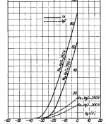
this one is not "empty" ... https://frank.pocnet.net/sheets/066/a/AL1.pdf
nor is this one : https://frank.pocnet.net/sheets/204/a/AL1.pdf
nor is this one : https://frank.pocnet.net/sheets/204/a/AL1.pdf
Hello!
Has anybody seen or have a model for the PCC85? The curves are not the same as for the ECC85.
Thanks!
Jose
Has anybody seen or have a model for the PCC85? The curves are not the same as for the ECC85.
Thanks!
Jose
Code:
* ==============================================================
* PCC85-2.4 LTSpice model
* Modified Koren model (8 parameters): mean fit error 0.119021mA
* Traced by Wayne Clay on 05/30/2018 using Engauge Digitizer and
* Cuvre Captor v0.9.1 from Philips data sheet
* Vg=-2.4 Vp=200 Ip=10mA S=6mA/V mu=46 Rp=7700
* ==============================================================
.subckt PCC85  P G K
    Bp  P K  I=
+ (0.03754423199m)*uramp(V(P,K)*ln(1.0+(-0.02799372538)+exp((1.140228068)+
+ (1.140228068)*((88.68943305)+(-2763.120627m)*V(G,K))*V(G,K)/sqrt((45.46362807)**2+
+ (V(P,K)-(21.00771062))**2)))/(1.140228068))**(1.222688513)
    Cgp G P 2.2p ; 0.7p added (1.5p)
    Cgk G K 3.8p ; 0.7p added (3.1p)
    Cpk P K 0.38p ; 0.2p added (0.18p)
    Cps P 0 1.0p ; Screen connected to ground
    Rpk P K 1G ; to avoid floating nodes
    d3  G K dx1
.model dx1 d(is=1n rs=2k cjo=1pf N=1.5 tt=1n)
.ends PCC85

* ==============================================================
* PCC85_Te LTSpice model
* Koren model (5 parameters): mean fit error 0.2441mA
* Traced by Wayne Clay on 06/17/2020 using Engauge Digitizer 10.10
* and Cuvre Captor v0.9.1 from Tesla data sheet
* Eg=-2.1V Ep=200 Ip=10mA S=5.8mA/V Mu=48
* ==============================================================
.subckt PCC85_Te  P G K
    Bp  P K  I=(0.05380690424m)*uramp(V(P,K)*ln(1.0+exp((1.342914016)+
+ (1.342914016)*(105.3430138)*V(G,K)/sqrt((1.544173159k)+
+ (V(P,K))**2)))/(1.342914016))**(1.152883537)
    Cgp G P 2.5p ; 0.7p added (1.85p)
    Cgk G K 4.0p ; 0.7p added (3.3p)
    Cpk P K 0.43p ; 0.2p added (0.23p)
    Cps P 0 1.4p ; Screen connected to ground
    Rpk P K 1G ; to avoid floating nodes
    d3  G K dx1
.model dx1 d(is=1n rs=2k cjo=1pf N=1.5 tt=1n)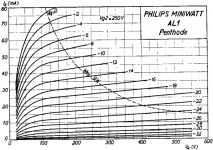
.ends PCC85_TeCan you find inter-electrode capacitance of AL1? Here is the pentode model:
Code:
**** AL1_P ******************************************
* Created on 01/27/2023 08:45 using paint_kip.jar
* www.dmitrynizh.com/tubeparams_image.htm
* Plate Curves image file: AL1-P.png
* Data source link: <plate curves URL>
*----------------------------------------------------------------------------------
.SUBCKT  AL1_P P G2 G K ; LTSpice tetrode.asy pinout
* .SUBCKT AL1_P P G K G2 ; Koren Pentode Pspice pinout
+ PARAMS: MU=8.24 KG1=4728.6 KP=90.91 KVB=164.51 VCT=1.56 EX=1.386 KG2=14484.19 KNEE=24.95 KVC=2.631
+ KLAM=1.562E-9 KLAMG=5.568E-4 KNEE2=31.53 KNEX=26.51  KNK=0.001563 KNG=7.097E-6 KNPL=47.5 KNSL=29.57 KNPR=47.5 KNSR=34.42
+ CCG=3P CGP=1.4P CCP=1.9P VGOFF=-0.6 IGA=0.001 IGB=0.3 IGC=8 IGEX=2
* Vp_MAX=550 Ip_MAX=80 Vg_step=4 Vg_start=0 Vg_count=15
* X_MIN=37 Y_MIN=29 X_SIZE=781 Y_SIZE=568 FSZ_X=1296 FSZ_Y=736 XYGrid=true
* Rp=1400 Vg_ac=20 P_max=9 Vg_qui=-28 Vp_qui=300
* showLoadLine=n showIp=y isDHP=n isPP=n isAsymPP=n isUL=n showDissipLimit=y
* showIg1=y isInputSnapped=y addLocalNFB=n
* XYProjections=n harmonicPlot=y dissipPlot=n
* UL=0.43 EG2=250 gridLevel2=y addKink=y isTanhKnee=y advSigmoid=n
*----------------------------------------------------------------------------------
RE1  7 0  1G    ; DUMMY SO NODE 7 HAS 2 CONNECTIONS
E1   7 0  VALUE=  ; E1 BREAKS UP LONG EQUATION FOR G1.
+{V(G2,K)/KP*LOG(1+EXP((1/MU+(VCT+V(G,K))/SQRT(KVB+V(G2,K)*V(G2,K)))*KP))}
RE2  6 0  1G    ; DUMMY SO NODE 6 HAS 2 CONNECTIONS
E2  6 0  VALUE={(PWR(V(7),EX)+PWRS(V(7),EX))} ; Kg1 times KIT current
RE21 21 0 1
E21  21 0 VALUE={V(6)/KG1*ATAN((V(P,K)+KNEX)/KNEE)*TANH(V(P,K)/KNEE2)} ; Ip with knee but no slope and no kink
RE22 22 0 1 ; E22: kink curr deviation for plate
E22  22 0 VALUE={V(21)*LIMIT(KNK-V(G,K)*KNG,0,0.3)*(-ATAN((V(P,K)-KNPL)/KNSL)+ATAN((V(P,K)-KNPR)/KNSR))}
G1   P  K  VALUE={V(21)*(1+KLAMG*V(P,K))+KLAM*V(P,K) + V(22)}
* Alexander Gurskii screen current, see audioXpress 2/2011, with slope and kink added
RE43 43 K 1G ; Dummy
E43  43 G2 VALUE={0} ; Dummy
G2   43 K  VALUE={V(6)/KG2*(KVC-ATAN((V(P,K)+KNEX)/KNEE)*TANH(V(P,K)/KNEE2))/(1+KLAMG*V(P,K))-V(22)}
RCP  P K  1G     ; FOR CONVERGENCE
C1   K G  {CCG}  ; CATHODE-GRID 1
C2   G P  {CGP}  ; GRID 1-PLATE
C3   K P  {CCP}  ; CATHODE-PLATE
RE23 G 0 1G
GG G K VALUE={(IGA+IGB/(IGC+V(P,K)))*(MU/KG1)*
+(PWR(V(G,K)-VGOFF,IGEX)+PWRS(V(G,K)-VGOFF,IGEX))}
.ENDS
*$
Attachments

- Home
- Amplifiers
- Tubes / Valves
- Vacuum Tube SPICE Models