I've had similar thoughts (and I have a similar problem only allowed two turntables in the house. She's only found two of the 5 in the shed). One of mine is a Roksan where the centre spindle can be removed so adjustment can be made. In theory once you knew the correction vector you could use a micrometer to nudge the record the required amount. But it's measuring the eccentricity to calculate that vector that is the issue.
I remember seeing the TX-1000 being demo'd on Tomorrow's world when it came out. Was very impressive to watch, but back then didn't realise how big an effect it might have on the sound.
I remember seeing the TX-1000 being demo'd on Tomorrow's world when it came out. Was very impressive to watch, but back then didn't realise how big an effect it might have on the sound.
It's nice when everything works.
Scott-
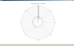
I'm running your polarplotrev3 script using Anaconda 5.0.1 (Python 3.6.3) and am getting a rather nasty glitch at the beginning of the plot, which throws off the scale. Any ideas on clearing this up?
Attachments
Scott-
I'm running your polarplotrev3 script using Anaconda 5.0.1 (Python 3.6.3) and am getting a rather nasty glitch at the beginning of the plot, which throws off the scale. Any ideas on clearing this up?
Sorry about that, it's one of those things. The IIR filter on the data has an initial transient which on most data sets is small because I start the filter at the mean frequency but on eccentric LP's you can catch an initial frequency far from the mean.
I will fix this for sure for a final release but in the meantime the fix was to just force the first 5 degrees or so of the plot to blank the glitch. If you can't manage the work around with this info I could go back and find the lines you need to change.
That's it, I was being slavish in getting my plots to line up exactly with LD's in reality the start point is arbitrary. We at one time were talking about lining up the plots to platter position, this is just a few degrees of offset.
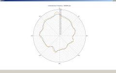
I notice this LP has a lot of off center eccentricity. There also seems to be that 9 cycles per rev from pulley eccentricity and 300RPM drive motor?
I notice this LP has a lot of off center eccentricity. There also seems to be that 9 cycles per rev from pulley eccentricity and 300RPM drive motor?
Last edited:
That's it, I was being slavish in getting my plots to line up exactly with LD's in reality the start point is arbitrary. We at one time were talking about lining up the plots to platter position, this is just a few degrees of offset.
I notice this LP has a lot of off center eccentricity. There also seems to be that 9 cycles per rev from pulley eccentricity and 300RPM drive motor?
The LP was Acoustic Sounds Ultimate Test Disc; visibly off center (held shell moves side to side). The pulley was from a machine shop that was having trouble getting the center bore concentric. I was hoping to use the app to measure my progress on the pulleys. I have some different ones to test, I'll post any interesting results.
Thanks for the help.
Thanks for the help.
You're welcome and thanks for another example of how this display technique is a great diagnostic, the problems just jump out.
When that happens, as it does, I enlarge the centre hole. Then manually centre the test record for a minimum of headshell motion.The LP was Acoustic Sounds Ultimate Test Disc; visibly off center (held shell moves side to side).
An off centre test record is pretty useless anyway, I figure.
Finally unboxed my test records from storage this week, after a few years in the wilderness...........
LD
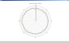
This is with a 600RPM BLDC motor, 3 belts and Jelco 750E 10" tonearm vs 300RPM AC synch, 1 belt and VPI 9" unipivot on previous plot.
I have the LP centered a little better (difficult to get it perfect). The stability seems better, within ±3Hz most of the time.
I have the LP centered a little better (difficult to get it perfect). The stability seems better, within ±3Hz most of the time.
Attachments

That looks good, once the ripples decorrelate it makes it more possible they are from the arm/cart resonance.
BTW if folks thought it was useful we could add filters to do the standard IEC wow and flutter tests, p-p and rms values.
BTW if folks thought it was useful we could add filters to do the standard IEC wow and flutter tests, p-p and rms values.
BTW if folks thought it was useful we could add filters to do the standard IEC wow and flutter tests, p-p and rms values.
Yes please!
And JIS please ?
If I could ask, and .exe too ?
I asked for some help on that, I don't have the resources to do that easily. As is I assume it works in any OS that has Python, even an RPi.
I'm an analogue engineer and haven't a clue on Python, apart from Monty, but then no one expects the Spanish Inquisition !
I added a 3rd plot to the display; a constant reference signal at 3150.0 Hz (displayed in black) that makes it easier to see the deviation from the reference (if3 and r3 in the code snippet):
Code:
freq1 = instfreq(sig,Fs,filter_freq)

if1 = freq1[2500:int(Fs*sec_per_rev)+2500]  # start 2500 samples in to prevent glitch at start up
if2 = freq1[int(Fs*sec_per_rev)+2500:int(2*Fs*sec_per_rev)+2500]
if3 = np.full(int(Fs*sec_per_rev),3150.0)  #create reference grid at 3150 Hz

maxf = int(max(max(if1),max(if2))+ Hz_per_tick)

r1 = 20.-(maxf-if1)/Hz_per_tick  #20 radial ticks at Hz_per_tick is fixed, adaptive scaling
r2 = 20.-(maxf-if2)/Hz_per_tick  #is an exercise for later
r3 = 20.-(maxf-if3)/Hz_per_tick

ax = plt.subplot(111, projection='polar')
ax.plot(theta,r1, color='tab:blue')
ax.plot(theta,r2, color='tab:orange')
ax.plot(theta,r3, color='black')
ax.set_rmax(20)
Attachments
ax = plt.subplot(111, projection='polar')
ax.plot(theta,r1, color='tab:blue')
ax.plot(theta,r2, color='tab😱range')
ax.plot(theta,r3, color='black')
ax.set_rmax(20)[/CODE]
That's a keeper. If people want to control colors, fonts, line weights, etc. maybe we could have a .init or .defaults text file? That is things like having 1000Hz or 3000Hz as reference would not involve modifying the code.
Last edited:
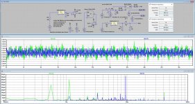
Just to compare results, I have entered in my LtSpice model the MK3wFpu1.wav file that was provided by JP, see #527 and #528 on page 53 of this thread.Thx - here's my edition of the polar plot for that file, starting at 10s.
Performance has, indeed, gone to the dogs through the act of measuring the FG signal, it seems.
Two spectral peaks in the WF file also seem to show up in the FG signal file, but by no means in the same ratio.............perhaps including the triangular like shape that isn't rotation synchronous...........
I agree, the FG monitoring method isn't good.
LD
The big advantage that I see in using LTSpice is that it is freeware and you don't need to have acces to Matlab nor do you need to have any programming experience with script languages like Python.
The other advantage is that you can examine signals at any detail in the time and frequency domains.
In this example I have analyzed 32,4 seconds or 18 LP revolutions.
The FM demodulator is steered by signal MOD to keep track of the signal coming from the LP.
After a first measuring step, average frequency turned out to be 2995Hz.
This figure was entered in A1 the FM demodulator as Mark=2995.
When letting LTSpice run for 32.4 sec, the signal MOD shows the deviation in time from the average 2995Hz, where 1mV equals 0.1% pitch deviation.
This signal is further processed by an IEC386 filter, as well as by the same filter preceded by a 0.55Hz notch filter to remove eccentricity from the LP.
With the absolute value of both IEC filtered signals, wow and flutter can be calculated as W&F=2*Sqrt(Vrms^2-Vavg^2) .
From the information visible in the image, IEC386 Wow+Flutter = 0.09% and 0.55Hz Notch filtered IEC386 wow+Flutter = 0.08%
This shows that IEC386 measurement in combination with notch filtering gives more accurate results.
This 0.08% is fairly good and only few people will hear pitch variation. Very good sets can go as low as 0.03%.
Also shown in the image is the FFT of both the MOD and the notch filtered IEC386 signals, resp in green and blue.
At 33 1/3 rev/min, first harmonic is at 0.55 Hz,
And indeed the first peak in green in the FFT spectrum is this 0.55Hz component , but there is also a second harmonic that is even stronger in amplitude, indicating that more eccentric processes are at work here.
The 0.55Hz component is effectively filtered by the notch filter as visible in blue, but the second harmonic at 1.1Hz is still visible although a factor 5 attenuated.
At 2.2Hz and at 3.3Hz there are also peaks, being exactly the 4th and the 6th harmonic of the 0,55 Hz platter rotation, and there is even a peak at 7.7 Hz which cannot be anything else but the 14th harmonic of the platter rotation.
So eccentricity is taking its part in this recording.
Then the other obvious frequency is at 9.5 Hz, being Fres of Arm/Cart and a small one at 19 Hz, being the second harmonic of Fres.
Then at last there is a peak at 41 Hz, from which I have no idea where it comes from.
Now looking at LD's frequency plot in #528, peaks at 1.1 Hz, 3.3 Hz, 7.7 Hz and 9.46 Hz are also clearly visible, although not as accurate.
But 2,2 Hz and 41 Hz are missing, the latter because LD's plot stops already at 40Hz.
So to my opininion LTSpice gives an excellent alternative to custom fit solutions with scripting languages.
Hans
Attachments
- Home
- Source & Line
- Analogue Source
- Turntable speed stabilty