Third bunch is about 100mm / 4" diameter piston driver with round over into infinite baffle
of radius 25mm / 1"


of radius 50mm / 2"


of radius 100mm / 4"


of radius 200mm / 8"


Michael
of radius 25mm / 1"
of radius 50mm / 2"
of radius 100mm / 4"
of radius 200mm / 8"
Michael
Fourth bunch is about 200mm / 8" diameter piston driver with round over into infinite baffle
of radius 25mm


of radius 50mm / 2"


of radius 100mm / 4"


of radius 200mm / 8"


Michael
of radius 25mm
of radius 50mm / 2"
of radius 100mm / 4"
of radius 200mm / 8"
Michael
Michael
Those thin, vertical lines of high pressure, that appear in the directivity plots with large diaphragms, what are those? What is causing them?
These are points of constructive interference (for a small frequency band at the listening distance and off axis angle shown) as a most basic explanation.
Remember that it's all about diffraction > reflection > delay > interference when it comes to sound field examination.
I like to look at these effect like to be kind of a virtual focus – without exactly knowing how to reverse engineering to be honest – maybe RCW or others can provide some interesting theorys or math about.
BTW there is a inverse of this effect seen quite often as a sharp recess in some other plots I have posted.
Michael
Last edited:
Those thin, vertical lines of high pressure, that appear in the directivity plots with large diaphragms, what are those? What is causing them?
Most likely those are numerical errors in the BEM caclulations which occur at interior resonances of the BEM problem. At these resonances the BEM problem becomes singular and highly unstable. Very sharp features like that would be impossible in the real world and hence can only be the result of a numerical problem. Basically just ignore those precise frequencies and look at either side and you can tell what would happen in between.
There is obviuosly some aliasing of the answers going on in the later sims.
Also in the later plots its apparent that the scale is clipped as there should be a continuous gradation of SPL and not a flat at the maximum level. I would also like to see a far lower range on the SPL plots, more like 30 dB than 50 dB.
Last edited:
Also in the later plots its apparent that the scale is clipped as there should be a continuous gradation of SPL and not a flat at the maximum level. I would also like to see a far lower range on the SPL plots, more like 30 dB than 50 dB.
You always get clipping either on top or on bottom - even worse if you narrow SPL range - pure physics, or math if you like.
I've deliberately choosen that range - and to keep it constant over the full matrix of simus - as I found it a good compromise to keep an visual overview.
Which plots are you specifically interested in Earl ? - and what range SPL wise would you like me to apply ? - if its not for all plots shown 😉 - no problem...
Michael
Last edited:
Most likely those are numerical errors in the BEM caclulations which occur at interior resonances of the BEM problem. At these resonances the BEM problem becomes singular and highly unstable. Very sharp features like that would be impossible in the real world and hence can only be the result of a numerical problem.
No, don't think its impossible to have narrow >10dB peaks or notches in real world - actually I faced such strange issues in some measurements as well.
But I agree that these specific ones might be as well artefacts to be ignored. Most certainly the very fine lines at the top end >15k are kind of what you are referring to.
Its always a balancing act to weight simulation effort (time) against accuracy - nothing new - and something we will not get rid of the next few thousand years or so...
Anyway - these simus are a valid guide line I offer (if we don't get too picky) - and final real world results we (hopefully) will see when I measure my next upcoming Dipole Horn - desiged with the conclusons in mind I drew out of that simus.
🙂
Michael
A good rule of thumb to use is that a flat piston has transitional behavoir at a frequency whos wavelength is root three times the piston radius.
Up to this limit the field is always Gaussian, i.e. it always has a central maximum and no other maxima.
As Earl observes above this we start to run into limitations inherant in boudary element methods.
rcw.
Up to this limit the field is always Gaussian, i.e. it always has a central maximum and no other maxima.
As Earl observes above this we start to run into limitations inherant in boudary element methods.
rcw.
A good rule of thumb to use is that a flat piston has transitional behavoir at a frequency whos wavelength is root three times the piston radius.
Up to this limit the field is always Gaussian, i.e. it always has a central maximum and no other maxima.
rcw.
Are you saying that the max frequency for a Gaussian beam from flat wavefronts roughly is:
9kHz for a 25mm / 1" diameter piston
4.5kHz for a 50mm / 2" diameter piston
2kHz for a 100mm / 4" diameter piston
1KHz for a 200mm / 8" diameter piston
500Hz for a 400mm / 16" diameter piston
I guess you are referring to radiation into 2Pi or 4Pi space? This would be pretty consitent with my simus shown in
http://www.diyaudio.com/forums/showpost.php?p=1891535&postcount=418
Well, as I have shown - or at least tried - without having explecitely explained yet - its all about alingnment of points of diffraction.
This means the same flat wave front of a certain diameter results in quite different soundfild defects with no round over to IB (or 4Pi space) in conrtrary to a carefully designed contour for the round over (horn).
From that my conclusion was that we possibly should re-define the task of designing horns as to align points of diffraction (the contour in summary) with the goal to get best possible time of arrival consistency (smooth sound field) for a certain directivity of desire
😉
As Earl observes above this we start to run into limitations inherant in boudary element methods.
rcw.
Did I got you right - why do you think BEM isnt capable to calculate accurate results above former limits???
This certainly isn't my experience with AxiDriver so far...
Michael
For a 25mm. piston the frequency is 15.89kHz., the radius times the square root of three.
If you look at the regions where the glitches occur you can see a distinct difference between the field in and outside the boundry between the duct and the infinite baffle.
Ideally the place inside the duct should be formulated as a finite element problem, the outside field by the boundary element.
In geophysical problems where the only data you can get is basically from boundaries, these glitches are dealt with by interpolation and statistical methods.
As Earl has pointed out what happens at the glitch is actually far more probably an average of what is happening either side of it, and the software might well have facilities for dealing with this in its more advanced facilities, I haven't investigated it myself however.
rcw.
For a 25mm. piston the frequency is 15.89kHz., the radius times the square root of three.
rcw.
Ok so my list should have its frequencies doubled
If you look at the regions where the glitches occur you can see a distinct difference between the field in and outside the boundry between the duct and the infinite baffle.
rcw.
Have the feeling I'm not looking at the same things than you refer to.
Could you please some further explain on an example?
Ideally the place inside the duct should be formulated as a finite element problem, the outside field by the boundary element.
rcw.
I've read this before – but I'm not really convinced.
Asking the developers about the limitations what's *exactly* being calculated by AxiDriver BEM Software I got the following answer:
"AxiDriver ist ein finite Elemente Simulator für die Akustik und ein Lumped Element Simulator für den elektro-mechanischen Teil. Auf der akustischen Seite ist die Grösse der finiten Elemente die einzige Approximation, ansonsten ist die Berechnung vollständig und beinhaltet alle Reflektionen und Interferenzen und sogar die Nahfeldeffekte."
"AxiDriver is a finite element simulator for acoustics and a lumped element simulator for the electro acoustic part.
For the acoustic part the width of the finite elements are the only approximation, despite that, the calculation is complete, including all reflections and interference and even near field effects."
In geophysical problems where the only data you can get is basically from boundaries, these glitches are dealt with by interpolation and statistical methods.
rcw.
Its fascinating that you bring in your unique point of view – though hard to digest sometimes 😉
Anyway – thanks for your patience in translating – this is a cool thing.
As Earl has pointed out what happens at the glitch is actually far more probably an average of what is happening either side of it, and the software might well have facilities for dealing with this in its more advanced facilities, I haven't investigated it myself however.
rcw.
Over the course when further comparing simus with measurements we hopefully might develop more confidence in this kind of simulations...
Michael
An illustration of this is here
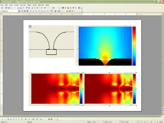
In this the major anomaly in the 4.7kHz. Region is shown on the top right hand.
As you can see there is a distinct difference between the plot inside the line that defines the baffle and that outside it.
I have purposely used this type of contour to exaggerate this type of effect, (the horn is a circular quadrant driven by a flat 20mm. Piston).
Although it has bad performance it is not quite as bad as this.
An this is illustrated by the two sonogram plots, these for a microphone distance of three metres.
The plot on the right is the raw one as calculated originally, and on the left is after being re sampled and smoothed using these facilities in vacs, the real performance would look a lot more like this.
Rcw.
An illustration of this is here
In this the major anomaly in the 4.7kHz. Region is shown on the top right hand.
As you can see there is a distinct difference between the plot inside the line that defines the baffle and that outside it.
I have purposely used this type of contour to exaggerate this type of effect, (the horn is a circular quadrant driven by a flat 20mm. Piston).
Although it has bad performance it is not quite as bad as this.
An this is illustrated by the two sonogram plots, these for a microphone distance of three metres.
The plot on the right is the raw one as calculated originally, and on the left is after being re sampled and smoothed using these facilities in vacs, the real performance would look a lot more like this.
Rcw.
RCW
Thanks for those, they make a good point. I have seen many things in these sims that simply don't make sense, you have shown one, I've seen others.
I did my PhD in numerical methods in acoustics and I'll tell you there are some real "gotcha's" possible and many many mistakes have been made by people with a significant expertise in the field, myself included. Basically you need to have confirmation of the sims or they really can be quite meaningless. There are many ways to do this, but simply accepting the results "as is" is totally wrong. They must be assumed to be wrong until proven that they are correct.
An illustration of this is here
In this the major anomaly in the 4.7kHz. Region is shown on the top right hand.
As you can see there is a distinct difference between the plot inside the line that defines the baffle and that outside it.
I have purposely used this type of contour to exaggerate this type of effect, (the horn is a circular quadrant driven by a flat 20mm. Piston).
Although it has bad performance it is not quite as bad as this.
An this is illustrated by the two sonogram plots, these for a microphone distance of three metres.
The plot on the right is the raw one as calculated originally, and on the left is after being re sampled and smoothed using these facilities in vacs, the real performance would look a lot more like this.
Rcw.
Ahh – now I understand - thanks.
Agree - of course, it always was clear that prior inside the horn there *must* be kept some degree of order if we want smooth sound field outside.
I've simpified it the way: "what is cooked inside the horn is spilled out into the room"
Your simu shown is pretty rough – it actually does not reflect the horns (roundover) property very well. If you look at my simus of 25mm Piston / 100 (200)mm round over you will see that they are much smoother.
No idea what you actually were after (besides giving a good example of artefacts) but for a pure horn behaviour you have to inject the flat wave front with *no* surround and make absolutely sure the contour starts where the diaphragm ends.
Otherwise you end up with a loooooot of artefacts - *not* caused by numerical problems - but by simple geometry.
Michael
Shouldn't good spherical wave front also have a very uniform pressure contour? I am a bit confused.
Quite a while back, when I posted this:
http://www.diyaudio.com/forums/showpost.php?p=1590534&postcount=1776
Earl's response was this:
http://www.diyaudio.com/forums/showpost.php?p=1590563&postcount=1777
Looking at polar pressure contour plots, I tend to feel that
An externally hosted image should be here but it was not working when we last tested it.
Really impressive, soongsc!
How big is the horn in your best attempt - the upper graph?
Michael
Last edited:
about 160mm deep from narrowest part of the throat to lip edge tangent to baffle, and 340mm diameter at the lip edge tangent to baffle.
Just listened to classical music
Big surprice
Sweet and smooth
VERY lifelike
And that is with just a 2.2uf series cap
No padding resistor
Yet it blends nicely with my ordinary 3way speakers
Easy on the ears
You know the "couldnt stop listening" experience
Well, thats for real
How can such a cheap combo can do that
Actually Im in serious doubt whether I should order the planned better drivers or just stick to this cheap McGee
I havent heard any other, so I have no idea about it
But this is a really big surprice to me
Last edited:
Just listened to classical music
But this is a really big surprice to me
Get a good nights sleep, everything will sound different in the morning.
- Home
- Loudspeakers
- Multi-Way
- Geddes on Waveguides