It is possible to gets posts temporarily unlocked for editing? I have made some posts in an informational thread and would like to make updates and fixes.
Hi Allen,
If possible, I would like the speakerbench posts (#8 to #22) unlocked for edits for roughly 48 hours in order to polish the text.
Thanks alot!
If possible, I would like the speakerbench posts (#8 to #22) unlocked for edits for roughly 48 hours in order to polish the text.
Thanks alot!
To make this work the way it needs to, I'd make two suggestions.
Firstly, post the replacement posts here, and I'll slot them into the thread.
Secondly, would you like to split this into a new thread beginning at (for example) Part 1? (and the other thread can link to it) The benefit is you'll have infinite edit time on the first post to make references and adjustments.
Great. In summary:
- I'll post all the replacement posts here (will take me a day or two)
- Yes, a new thread would be great (which the old thread can link to)
To be clear you'll remove old posts once I've finished posting new posts here?
- I'll post all the replacement posts here (will take me a day or two)
- Yes, a new thread would be great (which the old thread can link to)
To be clear you'll remove old posts once I've finished posting new posts here?
Yes, I'll treat these as replacements for the existing posts.
Would you like to create a fresh first post or do you want Part 1 to be the first post in the new thread?
Would you like to create a fresh first post or do you want Part 1 to be the first post in the new thread?
Using Part 1 as the first post is good -- particularly since it'll be editable.
Thanks alot for your help
Thanks alot for your help
Speakerbench -- part 4
Simple vs Advanced Model for Lossless Enclosures
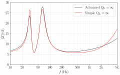
In order to illustrate the magnitude of the correction to be expected when using the advanced model, we present a box simulation example using the SEAS H1488-08 (L16RNX) midwoofer. Using Speakerbench, we model the SEAS driver in a vented box with volume Vb=26l and port tuning Fp=39.5Hz. All box losses (leakage, port, absorption) are taken to be negligible. Note that the 26l box (shown in part 1) was constructed for testing purposes only, with a removable baffle that accepts numerous drivers. As such it should not be considered to be an optimal box for the L16RNX.
In the attached figure we plot the total modeled system impedance in a lossless enclosure for the simple (red curve) and advanced (black curve) transducer models. The simple model exhibits the familiar result that both impedance peaks are nearly the same height. In contrast, the advanced model exhibits offset peaks, with the high-frequency (HF) peak increased in amplitude, and the low-frequency (LF) peak reduced in amplitude. This important asymmetry is a manifestation of the frequency-dependent viscoelastic damping.
Simple vs Advanced Model for Lossless Enclosures
In order to illustrate the magnitude of the correction to be expected when using the advanced model, we present a box simulation example using the SEAS H1488-08 (L16RNX) midwoofer. Using Speakerbench, we model the SEAS driver in a vented box with volume Vb=26l and port tuning Fp=39.5Hz. All box losses (leakage, port, absorption) are taken to be negligible. Note that the 26l box (shown in part 1) was constructed for testing purposes only, with a removable baffle that accepts numerous drivers. As such it should not be considered to be an optimal box for the L16RNX.
In the attached figure we plot the total modeled system impedance in a lossless enclosure for the simple (red curve) and advanced (black curve) transducer models. The simple model exhibits the familiar result that both impedance peaks are nearly the same height. In contrast, the advanced model exhibits offset peaks, with the high-frequency (HF) peak increased in amplitude, and the low-frequency (LF) peak reduced in amplitude. This important asymmetry is a manifestation of the frequency-dependent viscoelastic damping.
Attachments
Speakerbench -- part 5
Models vs Reality for Lossless Enclosures
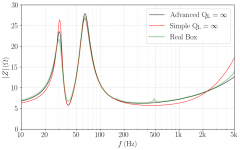
Without measuring the driver in a real enclosure, it is difficult to gauge the absolute accuracy of the simulations. In the attached figure, we measured the impedance of a midwoofer mounted in a real 26l enclosure, tuned to Fp=39.5Hz. The measured impedance is shown as the thick green curve. Of course the real enclosure is not perfectly lossless so we expect the impedance maxima to be reduced in height somewhat in comparison to the lossless simulations.
Note the measured HF peak (green) is above the simple model peak (red). We emphasize that there is no way to correct this result by adding losses to the simple model, as doing so will only reduce the peak height. On the other hand, the advanced model LF and HF peaks (black) are above the measured peaks (green), suggesting that better agreement may be achieved by adding box losses to the simulation.
Models vs Reality for Lossless Enclosures
Without measuring the driver in a real enclosure, it is difficult to gauge the absolute accuracy of the simulations. In the attached figure, we measured the impedance of a midwoofer mounted in a real 26l enclosure, tuned to Fp=39.5Hz. The measured impedance is shown as the thick green curve. Of course the real enclosure is not perfectly lossless so we expect the impedance maxima to be reduced in height somewhat in comparison to the lossless simulations.
Note the measured HF peak (green) is above the simple model peak (red). We emphasize that there is no way to correct this result by adding losses to the simple model, as doing so will only reduce the peak height. On the other hand, the advanced model LF and HF peaks (black) are above the measured peaks (green), suggesting that better agreement may be achieved by adding box losses to the simulation.
Attachments
Speakerbench -- part 6
Influence of Leakage Loss
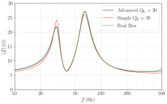
Although there are numerous potential loss channels (leakage, port, absorption), for simplicity we consider simulations with leakage loss only. This is the approach typically used by Small since it simplifies the analytic analysis. Setting QL = 30 in the simulations give the excellent advanced model result shown in the attached figure. This suggests a total enclosure loss no greater than QB ~ 30.
The critical observation is that, with QL = 30, the simple model still exhibits the LF/HF overshoot/undershoot of the lossless case. For this reason, it is difficult to estimate the true magnitude of the enclosure losses with the simple T/S model.
Influence of Leakage Loss
Although there are numerous potential loss channels (leakage, port, absorption), for simplicity we consider simulations with leakage loss only. This is the approach typically used by Small since it simplifies the analytic analysis. Setting QL = 30 in the simulations give the excellent advanced model result shown in the attached figure. This suggests a total enclosure loss no greater than QB ~ 30.
The critical observation is that, with QL = 30, the simple model still exhibits the LF/HF overshoot/undershoot of the lossless case. For this reason, it is difficult to estimate the true magnitude of the enclosure losses with the simple T/S model.
Attachments

Speakerbench -- part 7
Connection to Small's Rule
In assessing losses in practical enclosures, Richard Small (and previous authors) noticed that measured losses appeared to exceed theoretical expectations. Small inferred that even though the true leakage loss is insignificant, system losses somehow manifest as QL ~ 5-10 (Ref 1; references are given in Part 15). For this reason, an engineering rule of thumb emerged such that designers set QL = 7 for modeling purposes. This value was intended to broadly cover several types of losses (not only leakage but also absorption in the box). The analysis presented in the previous parts, however, leads us to suggest that the anomalous loss (correctly) observed by Small is a result not of the enclosure but of the driver -- specifically, driver viscoelasticity that is not included in the simple model. We further claim that corrections like Small's rule are not necessary (and not recommended) when using the advanced model.
Regarding accurate estimate of true losses, the simple model does not capture the asymmetry in the impedance peaks (as shown in Part 6). For this reason there is no obvious methodology to arrive at an accurate estimate of true enclosure losses using the simple model. With the advanced model, however, an accurate estimate of the true losses can be made.
Finally, it is well-known that measuring free-field frequency response at low frequencies is practically impossible (requiring a very large anechoic chamber). Conversely, measuring the impedance of a loudspeaker to very high precision is possible with low-cost equipment. By matching the measured to simulated impedance (as in Part 6), one can have confidence that the modeled low-frequency SPL is accurate and correctly includes all losses. Further, potential errors (for example, a real enclosure leak) are not easily identified in a frequency response measurement but will be readily apparent in an impedance measurement.
Speakerbench -- part 8
Community/Industry Acceptance of Advanced Parameters
Although transducer manufacturers are likely to have a Klippel analyzer in their laboratory, they rarely publish viscoelastic data. Measurement files from the Klippel analyzer are not readily available for download, and moreover, we do not know of any available software which can process this data and use it for box simulation. Claus initially thought that it would take a few years for some in the industry to adopt advanced parameters once the advantages were understood. Alas, 10 years after his presentation at a 2011 AES Convention in London (Ref 2), and although the work has caught the attention of both industry professionals and DIYers, few people do box simulation using the advanced model. Indeed, significant reformulations and software changes are required to move away from the simple T/S parameters.
Claus and I have advocated for some years for the acceptance of the advanced parameter description. To this end, we have published the relevant theoretical details, and have overcome certain obstacles; most notably, how to measure the viscoelasticity without expensive equipment (Ref 3), how to work with the advanced model in the time domain (Ref 5), and how to derive equivalent simple model parameters from the advanced parameters.
Speakerbench -- part 9
Speakerbench: A Free Community Web-App
The first step in the proposed modeling workflow is to compute the advanced model parameter set, and for this purpose we created the Dual-Added-Mass method. The details of this method are described in a recent AES article (Ref 3). The approach is verified to be capable of determining Bl within 1.0% and MMS within 2%. In particular, the viscoelastic parameter, β, as well as the advanced electrical parameters, are extracted from the measured data. The procedure offers a formal sanity-check for the measurement quality, unlike the classical added-mass method for which seasoned engineers would normally rely on experience and intuition to assess the quality of the extracted model parameters. Although the dual-added-mass procedure has been well-documented, it is non-trivial to design an algorithm to robustly carry out the parameter fitting and make an objective error estimate. Thus, to facilitate use and adoption of the advanced model, we have created a web-application named Speakerbench, available online at speakerbench.com. The user must only perform three impedance measurements with suitable equipment, and Speakerbench does the rest. The transducer data from the app is provided in JSON format (equivalent to a python dictionary) and can be downloaded and shared across the globe.
Unlike DLC Dumax, LinearX and Klippel data, the results from Speakerbench are valid only in the small-signal domain, but the data is of high quality and suitable for box design. After the advanced parameters are computed, the user can further carry out box simulations within Speakerbench, or export to dedicated design software, such as VituixCAD.
Speakerbench -- part 10
Steps In Creating An Advanced Transducer Model and Datasheet
The two requirements for good results with Speakerbench are (1) a sufficiently accurate setup for impedance measurements, and (2) a quality scale for measuring the added masses. Measuring impedance should either be executed with a stepped-sine where each measurement is allowed to stabilize, or alternatively in a slow sweep (say minimum 10 seconds and preferably with a sweep profile that gives you more time at the lower frequencies). Measuring with 0.1 gram precision is mandatory for normal transducers with MMS in the 10g-25g range.
Let's walk through the process.
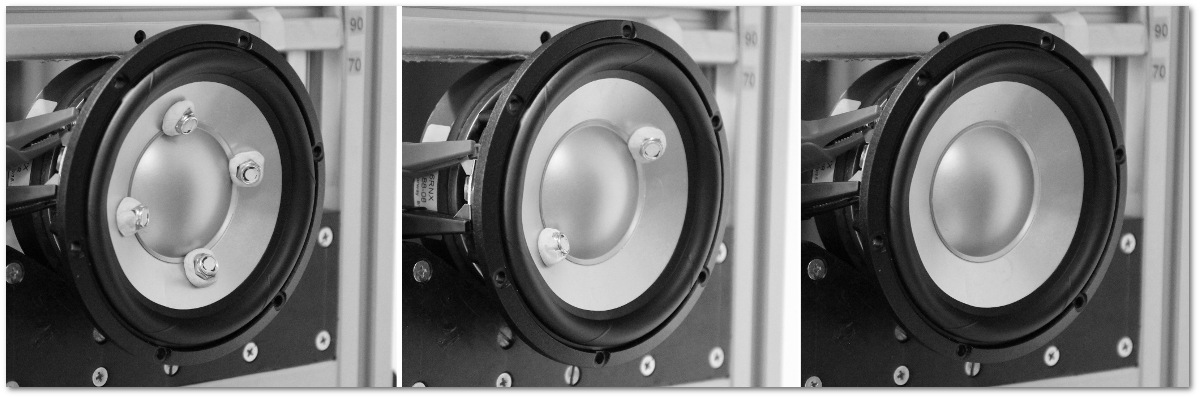
Collect 4 masses (using, for instance, a combination of Blu Tack and nuts) to be added to the diaphragm of the transducer. We recommend that total mass, which we denote by m2, be close to the moving mass of the driver. This is just a guideline and not essential. The progression of the driver measurements is shown in the image below:
STEPS
Steps In Creating An Advanced Transducer Model and Datasheet
The two requirements for good results with Speakerbench are (1) a sufficiently accurate setup for impedance measurements, and (2) a quality scale for measuring the added masses. Measuring impedance should either be executed with a stepped-sine where each measurement is allowed to stabilize, or alternatively in a slow sweep (say minimum 10 seconds and preferably with a sweep profile that gives you more time at the lower frequencies). Measuring with 0.1 gram precision is mandatory for normal transducers with MMS in the 10g-25g range.
Let's walk through the process.
Collect 4 masses (using, for instance, a combination of Blu Tack and nuts) to be added to the diaphragm of the transducer. We recommend that total mass, which we denote by m2, be close to the moving mass of the driver. This is just a guideline and not essential. The progression of the driver measurements is shown in the image below:
STEPS
- Attach the 4 masses, distributing them evenly near the voice coil (or just outside the area where the dust cap is attached) to ensure the load is balanced evenly to avoid rocking modes. This mass distribution is shown in the left panel in the image above.
- Measure the impedance of the transducer in free air, with all 4 pieces attached to the cone (left panel). This is the m2 impedance measurement.
- Gently remove two diagonal pieces such that about half the added mass remains on the cone (center panel). Remeasure the impedance with the remaining mass (m1) on the cone. For reference, weigh the removed mass (m2-m1) on a precision scale. When you remove the masses, avoid moving the cone (it should remain in its rest position).
- Gently remove the remaining two masses (right panel) and remeasure impedance. This is the unweighted measurement. Weigh the removed mass (m1) on a precision scale. Sum the two weights to calculate the total mass, m2.
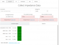
- Upload the three impedance measurements and the associated masses (m2 and m1) into the COLLECT app (see collect.png), then download the resulting JSON Z-file.
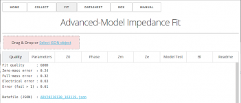
- Upload the Z-file from Step 5 into the FIT app (see fit.png). Speakerbench will then compute the advanced model parameters, as well as a quality of the fit metric that can be assessed in the resulting plot windows. The advanced parameters are provided in a downloadable JSON ADV-file.
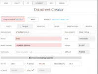
- Upload the ADV-file into the DATASHEET app (see creator.png). Here you simply add a description of the driver you've measured and a few important parameters, like SD and maybe XMAX, and the datasheet is then complete, provided in a downloadable JSON SBD-file.
Attachments
- Home
- Site
- Forum Problems & Feedback
- Unlocking posts for edits