Does anyone out there have working Python/Anaconda or Scilab code to read a PCM/wave file and convert to DSD?
For example, start with 44.1kHz 16 bit wave file and convert it to DSD256 or DSD512?
I ask as part of an educational effort related to a discrete DAC project.
For example, start with 44.1kHz 16 bit wave file and convert it to DSD256 or DSD512?
I ask as part of an educational effort related to a discrete DAC project.
Attachments
Don't know about those languages, but there is this: https://pcmdsd.com/Software/PCM-DSD_Converter_en.html ...Haven't tried it myself.
That said, there are some other PCM to DSD converter programs such as the Teac Converter and some paid programs. The ones I have tried didn't sound very good compared to what can be done with AK4137.
That said, there are some other PCM to DSD converter programs such as the Teac Converter and some paid programs. The ones I have tried didn't sound very good compared to what can be done with AK4137.
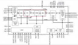
The encircled part of the block diagram looks like a sample rate converter rather than a PCM to DSD converter.
I have Pascal code for some sigma-delta modulators if it is of any use, the story goes that Python is similar to Pascal. It does not include a decent interpolation chain or a .wav file reading and .dsf file writing routine.
I have Pascal code for some sigma-delta modulators if it is of any use, the story goes that Python is similar to Pascal. It does not include a decent interpolation chain or a .wav file reading and .dsf file writing routine.
Korg Audiogate does that. There may be open-source software to do the same too, something like SRC- I forget the exact name.
The encircled part of the block diagram looks like a sample rate converter rather than a PCM to DSD converter.
Looks like AK4137 block diagram. The DSD modulator may be somewhere in the SRC block since PCM to DSD conversion doesn't work if SRC is bypassed by register settings.
Reading a wav file can be fairly simple if limited to support for CD rips. In that case there is a pretty simple explanation of what's in the header:...read a PCM/wave file...
https://docs.fileformat.com/audio/wav/
http://soundfile.sapp.org/doc/WaveFormat/
http://www.lightlink.com/tjweber/StripWav/WAVE.html
For more general info about wav files, the Wikipedia page is pretty good.
For large wav files, etc., there is a newer standard called RF64:
https://tech.ebu.ch/docs/tech/tech3306v1_1.pdf
Last edited:
The encircled part of the block diagram looks like a sample rate converter rather than a PCM to DSD converter.
I have Pascal code for some sigma-delta modulators if it is of any use, the story goes that Python is similar to Pascal. It does not include a decent interpolation chain or a .wav file reading and .dsf file writing routine.
Sure, if you post the Pascal code that could help me learn more.
So far I found a simple DSD64 example at github:
https://github.com/AUDIY/FPGA_PCM2DSD
If anyone downloads that example and wonders why nothing happens it is because one line of code is missing at the very end. Just add "plt.show()" to the end of the module.
I guess next I will see what I need to do to improve the example. I would like to get a quality DSD256 and/or DSD512 result (starting from red book CD in a wave file format).
Can anyone suggest a processing flow that I should consider? I would like to understand this subject much better and simulate the desired result in Python before I try to do anything with Quartus and my Altera Cyclone development board.
This is the simple starting example from github:
# -- coding: utf-8 --
"""
Created on Thu Dec 16 00:35:38 2021
@Author: AUDIY
"""
import numpy as np
import scipy.signal as signal
import matplotlib.pyplot as plt
# 1st-order Pulse Density Modulation
def PDM(x, nbits):
qe = 0 # Quantization Error
y = np.zeros(np.shape(x)[0]) # Return Array
# Modulation
for i in range(np.shape(x)[0]):
if x >= qe:
y = 1
else:
y = 0
# Maximize the Modulated Signal to PCM max Amplitude
yi_Analog = np.floor((((y*2 - 1) + 1)/2) * (2**nbits - 1) + 0.5) \
- (2 ** (nbits-1))
# Calcurate the Quantization Error
qe = qe + (yi_Analog - x)
return y.astype(int), qe
# float to Linear PCM Conversion
def LPCM(x, nbits):
#xmax = np.max(x) # Maximum float Amplitude
xmax = 1
#xmin = np.min(x) # Minimum float Amplitude
xmin = -1
# Quantization
x_LPCM = np.floor(((x - xmin)/(xmax - xmin)) * (2 ** nbits - 1) + 0.5) \
- (2 ** (nbits-1))
return x_LPCM.astype(int)
# Zero-order Hold Linear PCM Upsampling
def ZeroOrderHold(xPCM, OSR):
y = signal.upfirdn(np.ones(OSR), xPCM, OSR)
return y
# Main Entry Point
if name == "main":
print("Hello World")
# PCM parameters
fs_PCM = 44100 # Sampling frequency
nbits = 16 # Quantization Bits
# DSD Parameters
OSR = 64 # DSD vs PCM sampling frequency ratio
fs_DSD = fs_PCM * OSR # DSD Sampling frequency
# Time Plots
t_length = 1 # Time length (sec)
t = np.arange(0, 1, 1/fs_PCM)
# Reference Analog Signal (Amplitude Range = [-1, 1])
f = 1000 # Frequency
x = np.sin(2 * np.pi * 1000 * t) # float Sine wave
#x = np.zeros(fs_PCM) # Mute Data
# Analog to Linear PCM conversion
x_LPCM = LPCM(x, nbits)
# Zero Order Hold to Convert DSD
x_LPCM_Hold = ZeroOrderHold(x_LPCM, OSR)
# Convert PCM to DSD
y_DSD, qe = PDM(x_LPCM_Hold, nbits)
# Plot the filtered DSD Signal, Normalized PCM and DSD Signal
y_filtered = signal.upfirdn(np.ones(10), y_DSD) #Moving Average Filter
y_filtered = y_filtered/np.max(y_filtered) # Normalize
print("Before Plots")
plt.figure()
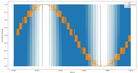
plt.plot(np.arange(0, 1, 1/fs_DSD)[0:2822], y_DSD[0:2822] * 2 - 1, label="DSD") # DSD
plt.plot(np.arange(0, 1, 1/fs_DSD)[0:2822], y_filtered[0:2822] * 2 - 1, label="Filtered DSD") # Filtered Data
plt.plot(np.arange(0, 1, 1/fs_DSD)[0:2822], x_LPCM_Hold[0:2822]/np.max(x_LPCM_Hold), label="PCM") # PCM
plt.legend(loc="upper right")
plt.xlabel("Time
plt.ylabel("Normalized Amplitude")
plt.show()
print("After Plots")
Attachments
You can find my Pascal code in this thread, starting at post #19:
https://www.diyaudio.com/community/...elta-dac-operation-wanted.311860/post-5180060
I posted several Pascal programs with various sigma-delta routines on that thread to clear up the OP's misunderstanding about the limitations of sigma-delta modulation.
For the idea behind it, see this article:
https://linearaudio.net/sites/linearaudio.net/files/03 Didden LA V13 mvdg.pdf
There is also some general information about sigma-delta modulation in it, and references to the most important articles.
You can find the Verilog versions of my modulators on the Downloads page of the Linear Audio site.
The Verilog version has a good interpolation chain, but it was generated with the Xilinx FIR compiler, so its source code is missing. The Pascal version only has linear interpolation, which is quite insufficient, but was good enough for the purpose of the thread I linked to.
Last edited:
Usually the process is to start with a CD rip, upsample the PCM using zero-stuffing followed by high quality LP filtering (Linear Phase FIR, Windowed Sinc, etc.). Filter coefficients may be adjusted to give the filter some needed gain. After that comes conversion to DSD. Converting 24/192 or 24/176.4 to DSD should produce a variant of DSD256. More or less the same process is using if converting to DSD using AK4137. The first one upsamples the PCM, the second AK4137 does the PCM->DSD256 conversion.
https://dspguru.com/dsp/faqs/multir... the process of,of the original sampling rate.
https://en.wikipedia.org/wiki/Upsampling
https://www.eetimes.com/multirate-dsp-part-1-upsampling-and-downsampling/
Regarding delta-sigma modulation, the sort of original bible on the subject is published by IEEE, and is sometimes referred to as the Green Book. The title is, "Understanding Delta-Sigma Data Converters." The first edition tried to take a more intuitive approach to the subject. The 2nd Edition is more formal in presentation. You might try looking around for that one online. The first edition so far as I know is only available in hardcopy. Both editions are nice to have. If you need more info feel free to PM, may have some articles, etc., if that might be helpful.
A brief introduction to PDM (which Sony called DSD): https://en.wikipedia.org/wiki/Pulse-density_modulation
Also, MarcelfdG's Tube Dac article at Linear Audio is well worth careful study.
Ultimate SQ depends on both upsamping and DSD modulator algorithms. They all sound different. To see for yourself you can download a trial version of HQ Player. There are various upsampling filters and modulator algorithms you can try.
The other thing I would say is that even if you find some upsampling and DSD conversion code, it won't be obvious how it works without some study of DSP.
Last edited:
The main issue with the simple example is that it is only first order, a first-order single-bit sigma-delta modulator with no dithering. That means not very effective noise shaping and lots of issues with idle tones and signal-dependent distortion products. It's a good place to start from an educational point of view, but the performance will be very bad.So far I found a simple DSD64 example at github:
https://github.com/AUDIY/FPGA_PCM2DSD
If anyone downloads that example and wonders why nothing happens it is because one line of code is missing at the very end. Just add "plt.show()" to the end of the module.
I guess next I will see what I need to do to improve the example. I would like to get a quality DSD256 and/or DSD512 result (starting from red book CD in a wave file format).
Can anyone suggest a processing flow that I should consider? I would like to understand this subject much better and simulate the desired result in Python before I try to do anything with Quartus and my Altera Cyclone development board.
This is the simple starting example from github:
# -- coding: utf-8 --
"""
Created on Thu Dec 16 00:35:38 2021
@Author: AUDIY
"""
import numpy as np
import scipy.signal as signal
import matplotlib.pyplot as plt
# 1st-order Pulse Density Modulation
def PDM(x, nbits):
qe = 0 # Quantization Error
y = np.zeros(np.shape(x)[0]) # Return Array
# Modulation
for i in range(np.shape(x)[0]):
if x >= qe:
y = 1
else:
y = 0
# Maximize the Modulated Signal to PCM max Amplitude
yi_Analog = np.floor((((y*2 - 1) + 1)/2) * (2**nbits - 1) + 0.5) \
- (2 ** (nbits-1))
# Calcurate the Quantization Error
qe = qe + (yi_Analog - x)
return y.astype(int), qe
# float to Linear PCM Conversion
def LPCM(x, nbits):
#xmax = np.max(x) # Maximum float Amplitude
xmax = 1
#xmin = np.min(x) # Minimum float Amplitude
xmin = -1
# Quantization
x_LPCM = np.floor(((x - xmin)/(xmax - xmin)) * (2 ** nbits - 1) + 0.5) \
- (2 ** (nbits-1))
return x_LPCM.astype(int)
# Zero-order Hold Linear PCM Upsampling
def ZeroOrderHold(xPCM, OSR):
y = signal.upfirdn(np.ones(OSR), xPCM, OSR)
return y
# Main Entry Point
if name == "main":
print("Hello World")
# PCM parameters
fs_PCM = 44100 # Sampling frequency
nbits = 16 # Quantization Bits
# DSD Parameters
OSR = 64 # DSD vs PCM sampling frequency ratio
fs_DSD = fs_PCM * OSR # DSD Sampling frequency
# Time Plots
t_length = 1 # Time length (sec)
t = np.arange(0, 1, 1/fs_PCM)
# Reference Analog Signal (Amplitude Range = [-1, 1])
f = 1000 # Frequency
x = np.sin(2 * np.pi * 1000 * t) # float Sine wave
#x = np.zeros(fs_PCM) # Mute Data
# Analog to Linear PCM conversion
x_LPCM = LPCM(x, nbits)
# Zero Order Hold to Convert DSD
x_LPCM_Hold = ZeroOrderHold(x_LPCM, OSR)
# Convert PCM to DSD
y_DSD, qe = PDM(x_LPCM_Hold, nbits)
# Plot the filtered DSD Signal, Normalized PCM and DSD Signal
y_filtered = signal.upfirdn(np.ones(10), y_DSD) #Moving Average Filter
y_filtered = y_filtered/np.max(y_filtered) # Normalize
print("Before Plots")
plt.figure()
plt.plot(np.arange(0, 1, 1/fs_DSD)[0:2822], y_DSD[0:2822] * 2 - 1, label="DSD") # DSD
plt.plot(np.arange(0, 1, 1/fs_DSD)[0:2822], y_filtered[0:2822] * 2 - 1, label="Filtered DSD") # Filtered Data
plt.plot(np.arange(0, 1, 1/fs_DSD)[0:2822], x_LPCM_Hold[0:2822]/np.max(x_LPCM_Hold), label="PCM") # PCM
plt.legend(loc="upper right")
plt.xlabel("Time")
plt.ylabel("Normalized Amplitude")
plt.show()
print("After Plots")
The DSD converter I linked to in the 2nd post of this thread is open source, but its in C++. Comments in the source files are mostly in Japanese, but google translate can convert them a little at a time into English. It looks to have pretty nice noise shaping from the graphs at the original link. Github sources are at: https://github.com/serieril/PCM-DSD_Converter
Also, wouldn't expect to find much in the way of useful code in an interpreted scripting language. There is some stuff for Matlab of course, but there is probably some entry level cost involved to work with DSD_Toolbox.
OTOH there is a free version of Microsoft C++ compiler.
Also, wouldn't expect to find much in the way of useful code in an interpreted scripting language. There is some stuff for Matlab of course, but there is probably some entry level cost involved to work with DSD_Toolbox.
OTOH there is a free version of Microsoft C++ compiler.
Last edited:
Yes, that simple example was accessible but very limited.
Noise shaping is going to be the topic of my reading/study next I guess.
Perhaps you can help explain a mystery to me. If I go to a store like Sweetwater Sound there is all kinds of equipment for music recording or mixing which contains delta sigma ADC and DAC. Yet it appears that the recording is done in PCM format. Then there is the editing software (such as Pro Tools which seems to be a standard) which as far as I can tell is entirely in PCM. Then after recording, editing and mixing is complete it appears that conversion to DSD gets involved at the point of mastering. I am not sure if it is the format used for 90% of mastering or what specific number. (I presume it was not used in any of the classic/older CD release albums.) But I am told that DSD is used for mastering and archiving. This leads me to my "mystery" or question. What is the standard (detailed algorithm with effective noise shaping, etc) which is used to convert the recorded/edited/mixed PCM into DSD after/in the mastering process?
I ask since as pointed out earlier a simple first-order conversion will have very bad performance/results. So the industry must have a well worked out and polished standard if it is being used for mastering and archiving? Is that published anywhere?
I saw a fifth-order sigma-delta modulator that Sony used for SACD in an AES article once. I will look it up. I don't know if everyone used that exact modulator for SACD.
Digital audio needs to be in PCM format for editing, applying effects, mixing, etc. Thus ProTools and other equivalent recording applications use PCM format.
For ADCs, most modern ones seem to operate in 'raw' mode, which is produced by a multi-bit delta-sigma modulator, but with only a few bits of resolution and at a very high sample rate. Some ADC chips can internally convert from raw to PCM, DSD, or other formats. Sometimes the conversion can be done externally such as in an FPGA.
To me at least, the main problem with PCM seems to be with the quality of DSP often applied to it in mixing and mastering, and in relation to dacs. For various reasons that likely have to do more with the physics of what can practically be manufactured into low-ish cost ICs, listening tests often suggest that operating dacs in DSD256 (or higher) mode sounds subjectively better.
Math and theory may seem to suggest that DSD is not optimal. Can't be properly dithered, for one thing. No reason PCM shouldn't be as good or better than DSD. So, what else is left except issues of practical implementation? PCM has three clocks all shuffling data around inside a dac chip (BCLK, LRCK, MCLK). All the clock edges have harmonics extending up to hundreds of MHz or higher. The clocks may all have their own jitter. Coupling of clock noise through the dac chip substrate can make its way into the output stage (hence part of the reason for developing AK4499EXEQ). PCM requires multiple switches and other components be matched close enough so that randomly substituting one for another can average out the mismatches well enough for human consumption. OTOH DSD needs at least one good switch but not necessarily more than that, and then some filtering. There is only one clock for DSD. Could be those sorts of things and others are part of the explanation. Don't really know for sure, but maybe something to consider.
Last edited:
I can't find the fifth-order Sony modulator on my computer. I know I have it on paper in the attic, but I can't access the attic right now.
A nice feature of DSD (or of any single-bit sigma-delta modulate, whether it meets the Philips/Sony DSD spec or not) is that you can decode it with a low-pass filter, no matter what the exact algorithm of the sigma-delta modulator was. You might get a bit more ultrasonic noise than you had hoped for when you use a very shallow filter with a high-order modulator, but that's all. I guess that's why some proposed using it for archiving.
Edit: I found it on a USB stick:

b1 = 1, b2 = 0.5, b3 = 0.25, b4 = 0.125, b5 = 0.0625, c2 = -0.001953125, c4 = -0.03125, see M. O. J. Hawksford, "Time-quantized frequency modulation, time-domain dither, dispersive codes, and parametrically controlled noise shaping in SDM", Journal of the Audio Engineering Society, vol. 52, no. 6, June 2004, or his reference 26: H. Takahashi and A. Nishio, "Investigation of practical 1-bit delta-sigma conversion for professional audio applications", presented at the 110th Convention of the Audio Engineering Society, paper 5393.
A nice feature of DSD (or of any single-bit sigma-delta modulate, whether it meets the Philips/Sony DSD spec or not) is that you can decode it with a low-pass filter, no matter what the exact algorithm of the sigma-delta modulator was. You might get a bit more ultrasonic noise than you had hoped for when you use a very shallow filter with a high-order modulator, but that's all. I guess that's why some proposed using it for archiving.
Edit: I found it on a USB stick:
b1 = 1, b2 = 0.5, b3 = 0.25, b4 = 0.125, b5 = 0.0625, c2 = -0.001953125, c4 = -0.03125, see M. O. J. Hawksford, "Time-quantized frequency modulation, time-domain dither, dispersive codes, and parametrically controlled noise shaping in SDM", Journal of the Audio Engineering Society, vol. 52, no. 6, June 2004, or his reference 26: H. Takahashi and A. Nishio, "Investigation of practical 1-bit delta-sigma conversion for professional audio applications", presented at the 110th Convention of the Audio Engineering Society, paper 5393.
Last edited:
The attachment was meant to become an appendix of the valve DAC article, but got skipped because the article was too long. It could be useful if you should want to design your own sigma-delta modulator. There are smarter ways to calculate coefficients, but this straightforward method works - the calculations only get a bit lenghty when the order is high.
For the record, when I wrote the Linear Audio article, I was under the impression that high-order single-loop sigma-delta modulators had been known since around 1990, but I later learned that Robert W. Harris already made them in the first half of the 1980's. See US patent US4509037 (application filed 1 December 1982, date of patent 2 April 1985) for details.
For the record, when I wrote the Linear Audio article, I was under the impression that high-order single-loop sigma-delta modulators had been known since around 1990, but I later learned that Robert W. Harris already made them in the first half of the 1980's. See US patent US4509037 (application filed 1 December 1982, date of patent 2 April 1985) for details.
Attachments
On Github there is an apparently very good delta-sigma toolbox easily installed by PIP however when I installed it I found that it did not function.
I also found that there were demos in Jupyter Notebooks. That is nice but what I really want is to be able to run code on my Python installation as part of my educational effort.
Next I found a fork of the deltasigma package which was "fixed" so I set about figuring out how to get PIP to install a fork. That turns out to be pretty easy fortunately.
Since others might want to try the deltasigma package (and run into the same little problems) I am posting this first example that I got running:
python-deltasigma
A port of the MATLAB Delta Sigma Toolbox based on free software and very little sleep
The python-deltasigma is a Python package to synthesize, simulate, scale and map to implementable topologies delta sigma modulators.
It aims to provide a 1:1 Python port of Richard Schreier's excellent MATLAB Delta Sigma Toolbox, the de facto standard tool for high-level delta sigma simulation, upon which it is very heavily based.
I also found that there were demos in Jupyter Notebooks. That is nice but what I really want is to be able to run code on my Python installation as part of my educational effort.
Next I found a fork of the deltasigma package which was "fixed" so I set about figuring out how to get PIP to install a fork. That turns out to be pretty easy fortunately.
Since others might want to try the deltasigma package (and run into the same little problems) I am posting this first example that I got running:
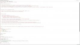
# KOZARD Cleanup/Fixing of NTF Synthesis - Demo #1
# August 8, 2022
#
# Cleanup/Fixing Needed Due To:
#
# 1. deltasigma is broken due to "AttributeError: module 'fractions' has no attribute 'gcd'"
# 2. Beginners might now know how to install a fork as opposed to the original (now unsupported and broken) package
# 3. The automated testing (NOSE) appears to also be broken even with the fixed/forked package
# 4. Many users want to use the examples and it might not be clear to beginners how to go from the Jupyter notebooks to working examples on their installation
#
#
#
# Philosophy of this Cleanedup/Fixed Demo:
#
# 1. Make no use of any additional complications for the beginners (NOSE, Jupyter, etc.)
# 2. Note all installation steps including fixing the broken package
#
#
#
# Getting Started:
#
# 1. Install Latest Python 3:
# - Goto https://www.python.org/downloads/
# - For Windows I Installed “python-3.10.5-amd64.exe”
# - Setup/Install Notes: Do Select "Add Python to Path"
# - Setup/Install Notes: Do Select "Install for All Users"
#
# 2. Install GIT so that you can later install the fixed fork of the deltasigma package
# - For Windows I went to: https://git-scm.com/download/win
# - Check installation from CMD with "git version" which replied "git version 2.37.1.windows.1" for my installation
#
# 3. Install the forked and fixed deltasigma package:
# - From CMD (run as admin) I used "pip install git+https://github.com/Y-F-Acoustics/python-deltasigma.git"
# - From the above you can see the location of the fork I used: "https://github.com/Y-F-Acoustics/python-deltasigma.git"
#
# 4. Run this module in IDLE (which should install in step 1.)
#
#
#
# After all of that the following "should" work fine assuming nothing else breaks between now (August 8, 2022) and when you try it
#
#
#imports
from future import division
from deltasigma import *
import numpy as np
import scipy as sp
import matplotlib.pyplot as plt
#
#
#start of example
order = 5
OSR = 32
#
#
# Synthesize
H0 = synthesizeNTF(order, OSR, opt=0)
#
# Plot the singularities
plt.subplot(121)
plotPZ(H0, markersize=5)
plt.title('NTF Poles and Zeros')
f = np.concatenate((np.linspace(0, 0.75/OSR, 100), np.linspace(0.75/OSR, 0.5, 100)))
z = np.exp(2j*np.pi*f)
magH0 = dbv(evalTF(H0, z))
#
#
# Plot the magnitude responses
plt.subplot(222)
plt.plot(f, magH0)
figureMagic([0, 0.5], 0.05, None, [-100, 10], 10, None, (16, 8))
plt.xlabel('Normalized frequency ($1\\rightarrow f_s)$')
plt.ylabel('dB')
plt.title('NTF Magnitude Response')
#
#
# Plot the magnitude responses in the signal band
plt.subplot(224)
fstart = 0.01
f = np.linspace(fstart, 1.2, 200)/(2*OSR)
z = np.exp(2j*np.pi*f)
magH0 = dbv(evalTF(H0, z))
plt.semilogx(f*2*OSR, magH0)
plt.axis([fstart, 1.2, -100,- 30])
plt.grid(True)
sigma_H0 = dbv(rmsGain(H0, 0, 0.5/OSR))
#plt.semilogx([fstart, 1], sigma_H0*np.array([1, 1]))
plt.semilogx([fstart, 1], sigma_H0*np.array([1, 1]),'-o')
plt.text(0.15, sigma_H0 + 5, 'rms gain = %5.0fdB' % sigma_H0)
plt.xlabel('Normalized frequency ($1\\rightarrow f_B$)')
plt.ylabel('dB')
plt.tight_layout()
# Always comically missing from beginner demos for some reason
plt.show()
Attachments


- Home
- Source & Line
- Digital Line Level
- Python/Anaconda or Scilab Code for PCM/Wave to DSD Conversion?