Here is the first part of the second demo: [KOZARD NTF Synthesis Demo 2A 5th Order LP Modulator]
# KOZARD Cleanup/Fixing of NTF Synthesis - Demo #2A
# August 22, 2022
#
#
#
# We wish to acknowledge and thank the authors:
# The demos are from "python-deltasigma" from G. Venturini, 2015
# The "Y-F-Acoustics" fork of "python-deltasigma" was used due to the 'fractions' module issue
# "python-deltasigma" is based on Richard Schreier's MATLAB Delta Sigma Toolbox
#
#
#
# A Little Bit of Cleanup/Fixing Was Needed Due To:
#
# 1. "python-deltasigma" is broken due to "AttributeError: module 'fractions' has no attribute 'gcd'"
# 2. Beginners might now know how to install a fork as opposed to the original (now unsupported and broken) package
# 3. The automated testing (NOSE) appears to also be broken even with the fixed/forked package
# 4. Many users want to use the examples and it might not be clear to beginners how to go from the Jupyter notebooks to working examples on their installation
#
#
#
# Philosophy of this Cleanedup/Fixed Demo:
#
# 1. Make no use of any additional complications for the beginners (NOSE, Jupyter, etc.)
# 2. Note all installation steps including fixing the broken package
#
#
#
# Getting Started:
#
# 1. Install Latest Python 3:
# - Goto https://www.python.org/downloads/
# - For Windows I Installed “python-3.10.5-amd64.exe”
# - Setup/Install Notes: Do Select "Add Python to Path"
# - Setup/Install Notes: Do Select "Install for All Users"
#
# 2. Install GIT so that you can later install the fixed fork of the deltasigma package
# - For Windows I went to: https://git-scm.com/download/win
# - Check installation from CMD with "git version" which replied "git version 2.37.1.windows.1" for my installation
#
# 3. Install the forked and fixed deltasigma package:
# - From CMD (run as admin) I used "pip install git+https://github.com/Y-F-Acoustics/python-deltasigma.git"
# - From the above you can see the location of the fork I used: "https://github.com/Y-F-Acoustics/python-deltasigma.git"
#
# 4. Run this Python module in IDLE development environment (which should have installed in step 1.)
#
#
#
# After all of that the following "should" work fine assuming nothing else breaks between now (August 22, 2022) and when you try it
#
#
#imports
from future import division
from deltasigma import *
import numpy as np
import scipy as sp
import matplotlib.pyplot as plt
#
#
#5th-order low-pass modulator
order = 5
OSR = 32
H = synthesizeNTF(order, OSR, 1)
#
#
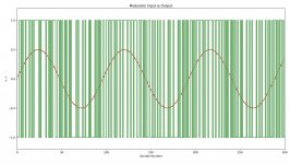
# First part of example
# Time-domain simulation with simulateDSM
# Test sine wave at ftest=(2/3)fb and amplitude of 0.5
plt.figure(figsize=(20, 4))
N = 8192
fB = int(np.ceil(N/(2.*OSR)))
ftest = np.floor(2./3.*fB)
u = 0.5*np.sin(2*np.pi*ftest/N*np.arange(N))
v, xn, xmax, y = simulateDSM(u, H)
t = np.arange(301)
plt.step(t, u[t],'r')
plt.step(t, v[t], 'g')
plt.axis([0, 300, -1.2, 1.2])
plt.xlabel('Sample Number')
plt.ylabel('u, v')
plt.title('Modulator Input & Output');
#
#
# NOTICE: Please close the plot window to continue the example!
plt.show()
#
#
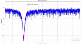
# Second part of example
# Output spectrum and SNR with calculateSNR
# Uses the output of the time domain simulation in the first part of the example, above
# The spectrum is computed through direct FFT of the time domain waveform and uses a Hann window
# Blue is the computed spectrum and magenta is the expected modulator transfer function in the frequency domain
#
# Example Fix: Replaced "N/2." with "N//2" (floor) due to TypeError: 'float' object cannot be interpreted as an integer
# Division / of integers yields a float, while floor division // of integers results in an integer.
f = np.linspace(0, 0.5, N//2 + 1)
spec = np.fft.fft(v * ds_hann(N))/(N/4)
#
# Example Fix (Again): Replaced "N/2." with "N//2" (floor) to get integer not float result for index
plt.plot(f, dbv(spec[:N//2 + 1]),'b', label='Simulation')
figureMagic([0, 0.5], 0.05, None, [-120, 0], 20, None, (16, 6), 'Output Spectrum')
plt.xlabel('Normalized Frequency')
plt.ylabel('dBFS')
snr = calculateSNR(spec[2:fB+1], ftest - 2)
plt.text(0.05, -10, 'SNR = %4.1fdB @ OSR = %d' % (snr, OSR), verticalalignment='center')
NBW = 1.5/N
Sqq = 4*evalTF(H, np.exp(2j*np.pi*f)) ** 2/3.
plt.plot(f, dbp(Sqq * NBW), 'm', linewidth=2, label='Expected PSD')
plt.text(0.49, -90, 'NBW = %4.1E x $f_s$' % NBW, horizontalalignment='right')
plt.legend(loc=4);
#
#
# NOTICE: Please close the plot window to continue the example!
plt.show()
#
#
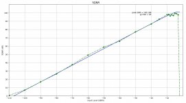
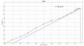
# Third part of example
# SNR versus Amplitude: prediction, simulation and peak extraction
#
# The "describing function method of Ardalan and Paulos" can be used since the example modulator is a binary (single-bit) structure
# This is done with predictSNR
# This is an approximate and quick method
#
# Next extended time simulations are done with simulateSNR
#
# Finally peakSNR is used to interpolate simulation results close to the SNR peak
# This results in an approximate value for peak SNR that could be expected by the syntesized modulator structure and its corresponding amplitude value
#
snr_pred, amp_pred, _, _, _ = predictSNR(H, OSR)
snr, amp = simulateSNR(H, OSR)
plt.plot(amp_pred, snr_pred, '-', amp, snr, 'og-.')
figureMagic([-100, 0], 10, None, [0, 100], 10, None, (16, 6),'SQNR')
plt.xlabel('Input Level (dBFS)')
plt.ylabel('SQNR (dB)')
pk_snr, pk_amp = peakSNR(snr, amp)
plt.text(-25, 85, 'peak SNR = %4.1fdB\n@ OSR = %d\n' % (pk_snr, OSR), horizontalalignment='right');
#
#
# NOTICE: Please close the plot window to continue the example!
plt.show()
#
#
Attachments
Here is the second part of the second demo: [Bandpass Modulator]
# KOZARD Cleanup/Fixing of NTF Synthesis - Demo #2B
# August 25, 2022
#
#
#
# We wish to acknowledge and thank the authors:
# The demos are from "python-deltasigma" from G. Venturini, 2015
# The "Y-F-Acoustics" fork of "python-deltasigma" was used due to the 'fractions' module issue
# "python-deltasigma" is based on Richard Schreier's MATLAB Delta Sigma Toolbox
#
#
#
# A Little Bit of Cleanup/Fixing Was Needed Due To:
#
# 1. "python-deltasigma" is broken due to "AttributeError: module 'fractions' has no attribute 'gcd'"
# 2. Beginners might now know how to install a fork as opposed to the original (now unsupported and broken) package
# 3. The automated testing (NOSE) appears to also be broken even with the fixed/forked package
# 4. Many users want to use the examples and it might not be clear to beginners how to go from the Jupyter notebooks to working examples on their installation
#
#
#
# Philosophy of this Cleanedup/Fixed Demo:
#
# 1. Make no use of any additional complications for the beginners (NOSE, Jupyter, etc.)
# 2. Note all installation steps including fixing the broken package
#
#
#
# Getting Started:
#
# 1. Install Latest Python 3:
# - Goto https://www.python.org/downloads/
# - For Windows I Installed “python-3.10.5-amd64.exe”
# - Setup/Install Notes: Do Select "Add Python to Path"
# - Setup/Install Notes: Do Select "Install for All Users"
#
# 2. Install GIT so that you can later install the fixed fork of the deltasigma package
# - For Windows I went to: https://git-scm.com/download/win
# - Check installation from CMD with "git version" which replied "git version 2.37.1.windows.1" for my installation
#
# 3. Install the forked and fixed deltasigma package:
# - From CMD (run as admin) I used "pip install git+https://github.com/Y-F-Acoustics/python-deltasigma.git"
# - From the above you can see the location of the fork I used: "https://github.com/Y-F-Acoustics/python-deltasigma.git"
#
# 4. Run this Python module in IDLE development environment (which should have installed in step 1.)
#
#
#
# After all of that the following "should" work fine assuming nothing else breaks between now (August 25, 2022) and when you try it
#
#
#imports
from future import division
from deltasigma import *
import numpy as np
import scipy as sp
import matplotlib.pyplot as plt
#
#
#Bandpass Modulator
f0 = 1./8
order = 8
OSR = 64
H = synthesizeNTF(order, OSR, 1, 1.5, f0)
#
#
# First part of example
# Time-domain simulation with simulateDSM
# Test sine wave at ftest=(1/3)fb and amplitude of 0.5
plt.figure(figsize=(20, 4))
N = 8192
fB = int(np.ceil(N/(2. * OSR)))
ftest = int(np.round(f0*N + 1./3 * fB))
u = 0.5*np.sin(2*np.pi*ftest/N*np.arange(N))
v, xn, xmax, y = simulateDSM(u, H)
t = np.arange(301)
plt.step(t, u[t], 'r')
plt.step(t, v[t], 'g')
plt.axis([0, 300, -1.2, 1.2])
plt.xlabel('Sample Number')
plt.ylabel('u, v')
plt.title('Modulator Input & Output');
#
#
# NOTICE: Please close the plot window to continue the example!
plt.show()
#
#
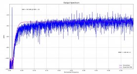
# Second part of example
# Output spectrum and SNR with calculateSNR
#
# Uses the output of the time domain simulation in the first part of the example, above
# The spectrum is computed through direct FFT of the time domain waveform and uses a Hann window
# Blue is the computed spectrum and magenta is the expected modulator transfer function in the frequency domain
#
# Example Fix: Replaced "N/2." with "N//2" (floor) due to TypeError: 'float' object cannot be interpreted as an integer
# Division / of integers yields a float, while floor division // of integers results in an integer.
f = np.linspace(0, 0.5, N//2 + 1)
spec = np.fft.fft(v * ds_hann(N))/(N/4)
#
# Example Fix (Again): Replaced "N/2." with "N//2" (floor) to get integer not float result for index
plt.plot(f, dbv(spec[:N//2 + 1]),'b', label='Simulation')
figureMagic([0, 0.5], 0.05, None, [-140, 0], 20, None, (16, 6), 'Output Spectrum')
f1 = int(np.round((f0 - 0.25/OSR) * N))
f2 = int(np.round((f0 + 0.25/OSR) * N))
snr = calculateSNR(spec[f1:f2+1], ftest - f1)
plt.text(0.15, -10, 'SNR = %4.1f dB @ OSR=%d)' % (snr, OSR), verticalalignment='center')
plt.grid(True)
plt.xlabel('Normalized Frequency')
plt.ylabel('dBFS/NBW')
NBW = 1.5/N
Sqq = 4*evalTF(H, np.exp(2j*np.pi*f))**2/3.
plt.plot(f, dbp(Sqq*NBW), 'm', linewidth=2, label='Expected PSD')
plt.text(0.475, -90, 'NBW=%4.1E x $f_s$' % NBW, horizontalalignment='right', verticalalignment='center')
plt.legend(loc=4);
#
#
# NOTICE: Please close the plot window to continue the example!
plt.show()
#
#
# Third part of example
# SNR versus Amplitude: prediction, simulation and peak extraction
#
# The "describing function method of Ardalan and Paulos" can be used since the example modulator is a binary (single-bit) structure
# This is done with predictSNR
# This is an approximate and quick method
#
# Next extended time simulations are done with simulateSNR
#
# Finally peakSNR is used to interpolate simulation results close to the SNR peak
# This results in an approximate value for peak SNR that could be expected by the syntesized modulator structure and its corresponding amplitude value
#
snr_pred, amp_pred, _, _, _ = predictSNR(H, OSR, None, f0)
snr, amp = simulateSNR(H, OSR, None, f0)
plt.plot(amp_pred, snr_pred, '-b', amp, snr, 'og-.')
figureMagic([-110, 0], 10, None, [0, 110], 10, None, (16, 6), 'SQNR')
plt.xlabel('Input Level (dBFS)')
plt.ylabel('SQNR (dB)')
pk_snr, pk_amp = peakSNR(snr, amp)
plt.text(-20, 95, 'peak SNR = %4.1fdB\n@ OSR = %d\n' % (pk_snr, OSR), horizontalalignment='right');
#
#
# NOTICE: This is a little slow. Be patient for the graph/plot to appear.
# NOTICE: Please close the plot window to continue the example!
plt.show()
#
#