What many people do not understand about horns is that most of their efficiency gain comes from the compression ratio, the horn load itself is a relatively minor effect. So going to 1:1 would simply be throwing away most of the gain

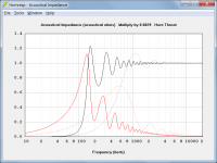
Hornresp clearly shows a 16 dB increase in spl @ 65 Hz between a direct radiator in a closed box and the same driver in a 1:1 C-R exponential horn with the same closed box encapsulation the back of the driver.

Do you disagree that the load impedances both go to zero at Low ka?
Do you disagree that both load impedances go to the same specific acoustic impedance at high frequencies?
If you agree to both those (which are facts, of course) then you must agree that at these two extremes then there cannot be any efficiency differences.
.
That's the electrical impedance.
The acoustic gain (output level) comes from the horn. I have some 4" throat horns here and some 5.25" drivers in a tuned enclosure. If I measure the response output of a 5.25" direct radiator and compare it with rigging the 4" throat (should be real close to 1:1) front horn to the same box (probably seal the port). I am guessing I'll see a 6-10 db gain over at least an octave.
I can also measure the impedance difference, they will be different (the horn should look a bit erratic) but the gain isn't coming from the electrical circuit, it's coming from the horn and it's better acoustic coupling to the air . I'll try it when I get a chance and post it here.
Hornresp clearly shows a 16 dB increase in spl @ 65 Hz between a direct radiator in a closed box and the same driver in a 1:1 C-R exponential horn with the same closed box encapsulation the back of the driver.
I'm not sure that I would buy this example in detail, but it does show what I was saying, no gain at LFs and no gain at HFs. Perhaps my estimate in the middle was a low. A lot of the gain in your test is from the resonance of the horn, i.e. the ripples. In a theoretical infinite horn this would not be so large.
And I would use an infinite baffle for the direct radiator since Horn response is most likely using that condition at the horns mouth (not knowing what the actual radiation would be for this device if it were not infinite baffle.)
Last edited:
That's the electrical impedance.
I'm not talking about the electrical impedance, I am talking about the acoustical impedance seen at the source due to the sound radiation. The power radiated will be the product of the radiation impedance (real part) and the source volume velocity squared. If the velocity is assumed to be independent of load, which it mostly is, then the power radiated will depend completely on the radiation impedance. The electrical impedance does not even enter into the problem in this regard.
I think that the sim shows what I was saying even if we might disagree on the details of the levels.
The gain from a 3 x compression ratio was exactly right as well, but this gain is across the whole bandwidth. (Ignoring the resonances which will change with CR)
Last edited:
If I get a chance I'll plot out the impedance on a piston with a and without a horn,
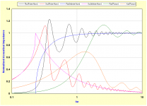
The dark traces show the normalised acoustical resistance (black) and normalised acoustical reactance (red) loading a rigid plane circular piston of area 500 cm2 coupled to a straight axisymmetric exponential horn having a throat cross-sectional area of 500 cm2, an axial length of 60 cm and a flare cutoff frequency of 100 hertz, with an infinite baffle at the horn mouth (half space radiation). The compression ratio is 1:1.
The light traces show the normalised acoustical resistance (grey) and normalised acoustical reactance (pink) loading the same piston mounted in an infinite baffle (half space radiation).
Attachments
Hi David, while I could argue the details of this, it is basically what I was saying, except I was talking about an infinite device where the resonances would not be so pronounced and I would have done the axis in dimensionless ka (that's always the way I think about things. ka here would be about 300-400 Hz where the difference is the greatest (again ignoring the resonance peaks.
I will admit at this point that I misspoke about the actual numbers in the region of maximum gain of a horn. When I thought about it later I could see that 1-2 dB was quite a low guess. My thinking was that the impedance would be about double at ka = .7, which would be twice the power and hence 4 times the SPL. This would be more like 12 dB - so clearly I had some brain freeze going one. The take away is that compression ratio is a factor across the useful bandwidth of a device while the horn gain is only over a limited bandwidth, nearly a decade (again, more than I had guessed at first.) However, for a waveguide designed mostly for directivity control, its useful range is well above ka = .7, so for a device like that, the horn gain is not as big a factor as the compression ratio. Since I never use horns at LFs or below ka = 1.0 this factor is what stuck in my mind.
One other question for you. You plot "Acoustic Power" which would be in watts, but the scale is the usual one for Sound Pressure. What do you use as a dB reference to get this to work out that way? There is a reference standard, but the dB levels would not be as you show.
Also, I assume that you are assuming a flat piston impedance for the mouth load impedance.
PS: Thanks for posting the analysis.
Last edited:
Hi Earl,
The chart was taken directly from Hornresp, which is why frequency rather than ka is shown. By exporting the data it is possible to convert to ka in Excel or similar. The attached chart shows the results for the same piston and horn as before, but with the x-axis now expressed in terms of ka, and scaled logarithmically. The infinite horn case has also been added.
The SPL at 1 metre due to radiated acoustical power is calculated in Hornresp as follows:
Given:
c = velocity of sound in air
rho = density of air
Ang = solid radiation angle in steradians (e.g. 2 * Pi for half space)
W = radiated acoustical power
S = area at 1 metre
I = sound intensity at 1 metre
p = sound pressure at 1 metre
pref = 20 micropascals
Then:
S = Ang
I = W / S
p = (I * rho * c) ^ 0.5
SPL = 20 * Log10(p / pref)
The appropriateness of the term "Acoustical Power" to describe the chart has been the source of much spirited discussion in the Hornresp thread. It all started with the post linked below 🙂.
http://www.diyaudio.com/forums/subwoofers/119854-hornresp-637.html#post4754696
Correct, taking the specified solid radiation angle into account.
You're most welcome 🙂.
Kind regards,
David
Hi David, while I could argue the details of this, it is basically what I was saying, except I was talking about an infinite device where the resonances would not be so pronounced and I would have done the axis in dimensionless ka (that's always the way I think about things. ka here would be about 300-400 Hz where the difference is the greatest (again ignoring the resonance peaks.
The chart was taken directly from Hornresp, which is why frequency rather than ka is shown. By exporting the data it is possible to convert to ka in Excel or similar. The attached chart shows the results for the same piston and horn as before, but with the x-axis now expressed in terms of ka, and scaled logarithmically. The infinite horn case has also been added.
One other question for you. You plot "Acoustic Power" which would be in watts, but the scale is the usual one for Sound Pressure. What do you use as a dB reference to get this to work out that way? There is a reference standard, but the dB levels would not be as you show.
The SPL at 1 metre due to radiated acoustical power is calculated in Hornresp as follows:
Given:
c = velocity of sound in air
rho = density of air
Ang = solid radiation angle in steradians (e.g. 2 * Pi for half space)
W = radiated acoustical power
S = area at 1 metre
I = sound intensity at 1 metre
p = sound pressure at 1 metre
pref = 20 micropascals
Then:
S = Ang
I = W / S
p = (I * rho * c) ^ 0.5
SPL = 20 * Log10(p / pref)
The appropriateness of the term "Acoustical Power" to describe the chart has been the source of much spirited discussion in the Hornresp thread. It all started with the post linked below 🙂.
http://www.diyaudio.com/forums/subwoofers/119854-hornresp-637.html#post4754696
Also, I assume that you are assuming a flat piston impedance for the mouth load impedance.
Correct, taking the specified solid radiation angle into account.
PS: Thanks for posting the analysis.
You're most welcome 🙂.
Kind regards,
David
Attachments
Ok then to me it is SPL, not "power".The appropriateness of the term "Acoustical Power" to describe the chart has been the source of much spirited discussion in the Hornresp thread. It all started with the post linked below 🙂.
Correct, taking the specified solid radiation angle into account.
I don't quite understand this. A flat piston in a rigid baffle - the only closed form solution for this type of problem - only has one solid radiation angle - Pi.
Also, we both know that the infinite exponential horn result that you show is fictitious. I would use an OS solution because it is theoretically correct (the exponential is not). In that case you would find that the two curves are almost identical except for a stretching along the ka axis. This is exactly how I have come to think about waveguides.
Last edited:
A flat piston in a rigid baffle - only has one solid radiation angle - Pi.
2 x Pi actually 🙂.
Yes, that's right 4 Pi for full field (it's solid angle not flat angle). But still how do you "take the specified solid radiation angle into account"? If it is always 2 PI then it can't be "specified".
But still how do you "take the specified solid radiation angle into account"?
Hornresp uses the traditional "piston in an infinite baffle" model to calculate the acoustical impedance per unit area at the horn mouth, but with the piston area given by Sp = 2 * Pi * Sm / Ang, where Sp is the piston area, Sm is the horn mouth area and Ang is the solid radiation angle. The model is used in those cases where plane wavefronts are assumed, and is based on the principle of acoustical images. Only when Ang = 2 * Pi does Sp = Sm.
When isophase wavefronts are assumed, Hornresp uses a different model to calculate the horn mouth impedance.
The plane wavefront mouth impedance model was developed almost 50 years (the first version of the simulation program that was to become Hornresp was written in Fortran IV and ran on a room-sized IBM mainfame computer). The Hornresp model pre-dates the work of Don Keele, who in his 1973 "Optimum Horn Mouth Size" paper assumed the conventional models of a rigid circular piston mounted in the end of a very long tube for full space, a rigid circular piston mounted in a flat infinite baffle for half space, and an infinite conical horn whose conical solid angle equals the radiation angle in question for fractional space.
The Hornresp model has proved over the years to be remarkably resilient, and more than adequate for bass horn simulations, which almost always assume plane wavefronts because of the low flare rates involved.
The plane wavefront mouth impedance model was developed almost 50 years (the first version of the simulation program that was to become Hornresp was written in Fortran IV and ran on a room-sized IBM mainfame computer).
The attachment shows one of the 80-column Hollerith input punch cards taken from the original source code listing. I still have the complete set of cards for the program - they are now close to 50 years old. The deck of cards making up the program is 8 cm thick. The actual Fortran IV code statement can be seen printed at the top of the card. It represents one line from the subroutine responsible for calculating the throat acoustical impedance of a finite conical horn.
Attachments
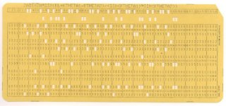
The attachment shows one of the 80-column Hollerith input punch cards taken from the original source code listing. I still have the complete set of cards for the program - they are now close to 50 years old. The deck of cards making up the program is 8 cm thick. The actual Fortran IV code statement can be seen printed at the top of the card. It represents one line from the subroutine responsible for calculating the throat acoustical impedance of a finite conical horn.
Very cool and interesting. 🙂
Hornresp uses the traditional "piston in an infinite baffle" model to calculate the acoustical impedance per unit area at the horn mouth, but with the piston area given by Sp = 2 * Pi * Sm / Ang, where Sp is the piston area, Sm is the horn mouth area and Ang is the solid radiation angle. The model is used in those cases where plane wavefronts are assumed, and is based on the principle of acoustical images. Only when Ang = 2 * Pi does Sp = Sm.
When isophase wavefronts are assumed, Hornresp uses a different model to calculate the horn mouth impedance.
The plane wavefront mouth impedance model was developed almost 50 years (the first version of the simulation program that was to become Hornresp was written in Fortran IV and ran on a room-sized IBM mainfame computer). The Hornresp model pre-dates the work of Don Keele, who in his 1973 "Optimum Horn Mouth Size" paper assumed the conventional models of a rigid circular piston mounted in the end of a very long tube for full space, a rigid circular piston mounted in a flat infinite baffle for half space, and an infinite conical horn whose conical solid angle equals the radiation angle in question for fractional space.
The Hornresp model has proved over the years to be remarkably resilient, and more than adequate for bass horn simulations, which almost always assume plane wavefronts because of the low flare rates involved.
At LFs almost any impedance works fine, but as the wavelengths approach the mouth size the radiation becomes very sensitive to the mouth impedance and a flat piston assumption is not going to work very well.
I too started with FORTRAN IV on IBM mainframes using cards and that was almost 50 years ago. I still use FORTRAN (Intel) for all my complex calculations, but I use VB.Net for the GUI. I have routines called from VB that are almost 50 years old.
I never understood LF horns so I haven't looked at them much. With amp power almost unlimited horn gain at LF is not really necessary and multiple subs works better anyways. But at HFs only a waveguide can control the directivity and so in that domain one has to understand how they work and simplistic assumptions like a flat piston mouth load don't cut it. In fact one can't even use Webster as it is not accurate enough. OS waveguide work so predictably that I have never used anything else. When something works you just stick with it.
Very cool and interesting. 🙂
Hi POOH,
You will recognize the code on the punch card as being the same as the first part of the denominator in the attached formula taken from Harry Olson's classic "Acoustical Engineering" text. It was the only reference book I had on horn loudspeakers when the original version of Hornresp was written. I didn't know it at the time, but it now seems likely that I may have been one of the early pioneers in simulating horn loudspeakers using a digital computer. The predicted response results were expressed in chart form, generated using alphanumeric characters, and printed out "sideways" on a high speed 132-character line printer. I still have some of the printouts 🙂.
Kind regards,
David
Attachments

anybody try newer acoustic modeling SW?
computer, solvers are a bit more sophisticated now
unfortunately free acoustic solver SW doesn't seem to have an obvious well supported project independent of proprietary GUI and awkward to build numeric packages, much less a nice Windows solution
but people are claiming few millions of elements in BEM or FDTD solvers run in tolerable time on today's PCs
I've been browsing, but not tried any yet:
Home - BEM acoustics
Product Overview - fastbem.com: The next generation BEM software!
k-Wave: A MATLAB toolbox for the time domain simulation of acoustic wave fields
Many many papers have been done using more advanced techniques. The most important that I know of is the PhD thesis of some guy in Australia (sorry don't recall his name.) He used an optimization routine to find that waveguide contour that gave the best polar response. It was a great piece of work.
The thing is that his results basically confirmed what I had found using closed form solutions of the wave equation (i.e. not numerical). The "best shapes" that he found were virtually identical to an OS waveguide with a large mouth flare.
Numerical solutions are fine, but sometimes just jumping into a problem using a numerical code isn't the best solution. Computers always give you an answer, but often times its the question that was wrong.
I may have been one of the early pioneers in simulating horn loudspeakers using a digital computer.
That may be true, but since you didn't give any dates, I am not sure. I published a paper on modeling compression drivers, including the horn, in JAES back in the late 70's early 80's (don't recall the exact date), so that's pretty early as well.
Many many papers have been done using more advanced techniques. The most important that I know of is the PhD thesis of some guy in Australia (sorry don't recall his name.)
Richard C. Morgans - "Optimisation Techniques for Horn Loaded Loudspeakers".
- Home
- Loudspeakers
- Multi-Way
- High vs. low compression ratio in horns