MI Pro v3.9 link to references & new v3.9 users manual
Hello Chris et al,
Thank you for your kind note. Please don't forget to also check out this URL to get great references on the use of MI Pro too:
Applications of Multi-Instrument Virtual Instrumentation Systems | Virtins Technology
Please also note the newly updated MI Pro 460 page users manual that is exceptionally extensive and addresses all of the extensive updates to the v3.9 version of MI Pro. Here are the specific links to two of the relevant MI Pro documents:
https://www.virtins.com/Multi-Instrument-Brochure.pdf
https://www.virtins.com/Multi-Instrument-Manual.pdf
Please note that when you download the newest version of MI Pro the download itself does come with this new users manual (and other PDF documentation as well) but I have provided the specific URL link here for those whom may not (yet) own MI Pro but simply would like to review the users manual for it without having to download the entire MI Pro setup program.
For those of whom may not yet know about MI Pro audio measurement software and its reputation, please see:
Practical Test & Measurement: The Virtins Multi-Instrument Software | audioXpress
With respect to the above URL link, please scroll down to the "Summing Up" to see how MI Pro was (is) rated as being far more powerful than other excellent audio measurement software such as ARTA, AudioTester, etc. (I own licensed versions of all the others, and I love them too, but overall, MI Pro simply does a lot more by comparison). Shown below are the key take aways from this excellent AudioXpress review:
Summing Up
Multi-Instrument is a stunningly versatile and capable software package. It is far more complex and difficult to use than most hobbyist-oriented software (e.g., ARTA or AudioTester) and costs significantly more. But the price is reasonable compared to professional packages, and the capabilities far exceed the simpler software. The simpler and less expensive software will likely take care of 80% of your needs, but once you have climbed the learning curve for Multi-Instrument, your measurement power will be an order of magnitude greater.
I will confess that writing this review was delayed again and again as I’d discover a new feature or a new way to use existing ones. I still think that I haven’t used more than 5% of Multi-Instrument’s capability. My procrastination was aided by an excellent set of application videos that Virtins has produced for its YouTube channel.
Finally, please note the far more recent 15 Apr 2020 AudioXpress article, again by the exceptionally knowledgeable reviewer Stuart Yaniger, where he states:
"...In a forthcoming article, I will discuss a software product that will also improve measurement capabilities, the latest version of Virtins Multi-Instrument..." (see: Fresh From the Bench: The Linear Audio Autoranger Mk II Measurement Interface | audioXpress)
This upcoming AudioXpress promised review will address the newer features of MI Pro v3.9 and it should be very interesting reading to see Stuart's keen insights and comments on the many new add-ons that the MI Pro v3.9 upgrade offers!
Have a great day!
MI Pro
6. Cumulative Spectral Decay (CSD)
View attachment 836930
This screenshot shows an impulse response (IR) that is 20 ms long and a CSD that spans 19.9 ms or so. The last line of the CSD therefore corresponds to the last 0.1 ms of the impulse response. The Fourier transform of this 0.1 ms long piece would have the lowest non-DC frequency bin at 2/0.1ms = 20 kHz, and the frequency resolution is also 20 kHz. However, the CSD plot in the screenshot is very different, as it shows frequency bins at low frequencies and high resolution throughout the entire time span. What's going on with this CSD?
Thank you for your comments, @mbrennwa.
Actually the total time length of the impulse response in that screenshot is 6314 / 44100 = 0.14317s =143.17ms not 20 ms, as indicated by “ ‘Point’ = 6314 ” at the top right of the screenshot. The oscilloscope window shows only the left most 20ms of total time length and there is actually a horizontal scrollbar at the bottom of the oscilloscope window. But that scrollbar is mostly covered by the Spectrum 3D Plot window to save a little more space for the presentation (sorry for this illusion🙂). The actually data used for that particular CSD contain 1024 samples (= FFT Size or initial window width) which spans the left-most 1024 / 44100 = 0.02322 s = 23.22ms. The CSD Sweep Range (see definition in the figure below) is set to 90% of the initial window width, that is 0.9*23.22 ms = 20.90 ms (Note: the labelled "19.9ms" in that screenshot is not the maximum one). Therefore the time length of the data used in the last spectral profile is about (23.22-20.90) = 2.32 ms. The lowest resolvable frequency is then about 1 /(2.32ms) =0.431kHz, which is correctly reflected in the CSD in that screenshot.
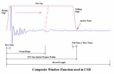
Actually the total time length of the impulse response in that screenshot is 6314 / 44100 = 0.14317s =143.17ms not 20 ms, as indicated by “ ‘Point’ = 6314 ” at the top right of the screenshot. The oscilloscope window shows only the left most 20ms of total time length and there is actually a horizontal scrollbar at the bottom of the oscilloscope window. But that scrollbar is mostly covered by the Spectrum 3D Plot window to save a little more space for the presentation (sorry for this illusion🙂). The actually data used for that particular CSD contain 1024 samples (= FFT Size or initial window width) which spans the left-most 1024 / 44100 = 0.02322 s = 23.22ms. The CSD Sweep Range (see definition in the figure below) is set to 90% of the initial window width, that is 0.9*23.22 ms = 20.90 ms (Note: the labelled "19.9ms" in that screenshot is not the maximum one). Therefore the time length of the data used in the last spectral profile is about (23.22-20.90) = 2.32 ms. The lowest resolvable frequency is then about 1 /(2.32ms) =0.431kHz, which is correctly reflected in the CSD in that screenshot.

Actually the total time length of the impulse response in that screenshot is 6314 / 44100 = 0.14317s =143.17ms not 20 ms, ... The actually data used for that particular CSD contain 1024 samples (= FFT Size or initial window width) which spans the left-most 1024 / 44100 = 0.02322 s = 23.22ms. The CSD Sweep Range (see definition in the figure below) is set to 90% of the initial window width, that is 0.9*23.22 ms = 20.90 ms (Note: the labelled "19.9ms" in that screenshot is not the maximum one). Therefore the time length of the data used in the last spectral profile is about (23.22-20.90) = 2.32 ms. The lowest resolvable frequency is then about 1 /(2.32ms) =0.431kHz, which is correctly reflected in the CSD in that screenshot.
Ah, ok, I see. This would mean that in the last line of the CSD, the first data point would be at 431 Hz, the second point at 862 Hz, the third at 1293 Hz, etc. Looking closely at the CSD plot, you can see that this is not the case. The first data point is about 380 Hz, and the data/curve resolution is much higher than 431 Hz. How can this be?
Good questions.
1. Apparent FFT frequency resolution vs Real FFT frequency resolution
The real FFT frequency resolution is equal to 1/T , where T is the time length of the data used in FFT.
The apparent FFT frequency resolution is equal to [Sampling Rate] / [FFT Size].
In CSD, the time length of the data used in FFT dwindles as the start side of the data window moves along the time axis. As a result, the real FFT frequency resolution becomes coarser along the way. On the other hand, the apparent FFT frequency resolution remains unchanged as the FFT size is kept constant through zero padding during the sliding process. Nevertheless, the deterioration of the frequency resolution can still be observed because zero padding in effect is equivalent to interpolation.
To answer this, I must use a more precise method with an accuracy of 1 data sample.
In CSD, when the start side of the data window slides along the time axis, there is another parameter – “Overlap Percentage” (see the definition in the figure below) which is used to control the sliding step.
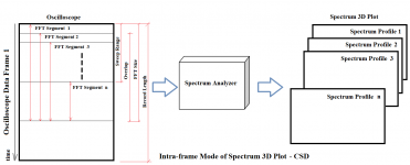
The number of spectral profiles in CSD is determined by:
[Number of Spectral Profiles] = 1+[Sweep Range] / ([FFT Size]-[Overlap Size])
where:
[Sweep Range] = [FFT Size] × [Sweep Percentage]
[Overlap Size] = [FFT Size] × [Window Overlap Percentage]
In that CSD example, [FFT Size] =1024, [Sweep Percentage] =90%, [Overlap Size] =99%, then:
[Sweep Range] = 1024 × 90% =921, [Overlap Size] = 1024 × 99% =1013, [Number of Spectrum Profiles]: 1 + 921 / (1024-1013) = 84 (as shown at the bottom in that CSD screenshot).
The sliding step is then: 1024-1013=11 (samples). This means that the last spectral profiles uses only 1024-(84-1) × 11 = 111 samples. The real frequency solution of the last spectral profile is then: 44100/111 = 397.3 (Hz). The apparent FFT frequency resolution is 44100 / 1024 = 43.07 Hz. The center frequency of the two FFT bins around 397.3Hz is 9×43.07 = 388Hz and 10×43.07 = 431Hz. The software has chosen the better one: 388Hz as the starting frequency of the CSD. I must say your estimation of 380Hz by simply looking at the small graph is very accurate indeed. 🙂
This would mean that in the last line of the CSD, the first data point would be at 431 Hz, the second point at 862 Hz, the third at 1293 Hz, etc. Looking closely at the CSD plot, you can see that this is not the case. The first data point is about 380 Hz, and the data/curve resolution is much higher than 431 Hz. How can this be?
1. Apparent FFT frequency resolution vs Real FFT frequency resolution
The real FFT frequency resolution is equal to 1/T , where T is the time length of the data used in FFT.
The apparent FFT frequency resolution is equal to [Sampling Rate] / [FFT Size].
In CSD, the time length of the data used in FFT dwindles as the start side of the data window moves along the time axis. As a result, the real FFT frequency resolution becomes coarser along the way. On the other hand, the apparent FFT frequency resolution remains unchanged as the FFT size is kept constant through zero padding during the sliding process. Nevertheless, the deterioration of the frequency resolution can still be observed because zero padding in effect is equivalent to interpolation.
The first data point is about 380 Hz
To answer this, I must use a more precise method with an accuracy of 1 data sample.
In CSD, when the start side of the data window slides along the time axis, there is another parameter – “Overlap Percentage” (see the definition in the figure below) which is used to control the sliding step.

The number of spectral profiles in CSD is determined by:
[Number of Spectral Profiles] = 1+[Sweep Range] / ([FFT Size]-[Overlap Size])
where:
[Sweep Range] = [FFT Size] × [Sweep Percentage]
[Overlap Size] = [FFT Size] × [Window Overlap Percentage]
In that CSD example, [FFT Size] =1024, [Sweep Percentage] =90%, [Overlap Size] =99%, then:
[Sweep Range] = 1024 × 90% =921, [Overlap Size] = 1024 × 99% =1013, [Number of Spectrum Profiles]: 1 + 921 / (1024-1013) = 84 (as shown at the bottom in that CSD screenshot).
The sliding step is then: 1024-1013=11 (samples). This means that the last spectral profiles uses only 1024-(84-1) × 11 = 111 samples. The real frequency solution of the last spectral profile is then: 44100/111 = 397.3 (Hz). The apparent FFT frequency resolution is 44100 / 1024 = 43.07 Hz. The center frequency of the two FFT bins around 397.3Hz is 9×43.07 = 388Hz and 10×43.07 = 431Hz. The software has chosen the better one: 388Hz as the starting frequency of the CSD. I must say your estimation of 380Hz by simply looking at the small graph is very accurate indeed. 🙂
Last edited:
...the apparent FFT frequency resolution remains unchanged as the FFT size is kept constant through zero padding during the sliding process.
I see, you are padding the data with zeros before applying the Fourier transform. I prefer not to do this because it results in a higher apparent resolution (as you explained in your post). I think this is misleading, because it does not show the raw data as it is. It might be useful to annotate the CSD plots accordingly so people know that they are looking at somewhat "fictional" data resulting from Fourier interpolation / zero padding.
I prefer not to do this because it results in a higher apparent resolution (as you explained in your post). I think this is misleading, because it does not show the raw data as it is. It might be useful to annotate the CSD plots accordingly so people know that they are looking at somewhat "fictional" data resulting from Fourier interpolation / zero padding.
Thank you for the discussion.
I think a higher apparent resolution resulting from zero padding is an advantage rather than a disadvantage here. It does not introduce fictional frequency components, but rather it provides denser spectral lines and eases the so-called “picket fence effect” issue. The signal here is not periodic and is time limited. The Fourier transform of N-point discrete-time samples in time domain (called DTFT, Discrete-Time Fourier Transform) is thus a continuous function of frequency. Sampling DTFT in the frequency domain yields DFT (Discrete Fourier Transform) and its faster version FFT. This frequency domain sampling can be of any points. The common DFT and FFT algorithm happen to use the same number of points as that in the time domain for the purpose of easy calculation and convenience, i.e. N points in the time domain yields N points in the frequency domain. It possible to make use of the common DFT or FFT algorithm to extract more than N points from the same continuous DTFT function. The way of doing it is zero-padding. In other words, FFT with and without zero padding are both extracted from the same DTFT function but with different sampling intervals in frequency.
The following two screenshots show an extreme case where zero-padding is a must to ease the picket fence effect in order to reveal the true spectrum of the data. The data in the time domain is a 1024-point Hann window. The first screenshot uses a 1024-point FFT while the second one uses a 1048576-point FFT. In the second screenshot, 1048576-1024 =1047552 zeros are padded at the end of the raw data in the time domain.
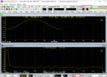
[Record Length] = 1024, [FFT Size] = 1024, i.e. no zero padding.
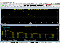
[Record Length] = 1024, [FFT Size] = 1048576, i.e. 1047552 zeros paded.
Obviously, the second one is the well-known spectrum of a Hann window. The first one happens to sample exactly at the troughs of the real Hann window spectrum as shown by the cyan reference curve in the second screenshot and thus creates an illusion.
Back to the CSD plot, zero padding is the defato implementation in various CSD software, even only for the purpose of speeding up. With a sliding step of only one or a few data samples, much slower DFT instead of FFT will have to be used if zero padding is not used. Moreover, different fractional octave smoothing and window functions are usually used in CSD. They will change the outlook of the CSD more drastically than zero-padding.
No fractional octave smoothing is applied in that CSD plot, but it can be applied if needed.
I think a higher apparent resolution resulting from zero padding is an advantage rather than a disadvantage here. It does not introduce fictional frequency components,...
It DOES introduce fictional frequency components! As you wrote, the resolution of the Fourier transform data is 1/T. If the result has higher resolution, data was added that is not in the original raw data. That's what I mean by "fictional".
...but rather it provides denser spectral lines...
Sure, the CSD looks "nicer". But it's misleading, because it shows fictional data. Just plot the CSD without the zero-padding touch-up. In many cases you'll realise that the fence simply is not there. I fell for this more than once.
I believe the point is that the fence is actually there - it is the transfer of the window used.
Jan
Jan
Sure, the CSD looks "nicer". But it's misleading, because it shows fictional data. Just plot the CSD without the zero-padding touch-up.
It looks like that you still consider the N-point discrete samples extracted from the continuous DTFT function of the N-point raw data as the “true” spectrum, despite the fact that the (N+M)-point discrete samples extracted from the same DTFT have a better channel to reflect the true spectrum from probability point of view.
Ok, let’s follow your way temporarily here. In CSD, you will have to connect these sparse N-point discrete spectral samples on the screen to make the spectrum look continuous. If you use straight lines, you are using linear interpolation between them. As both the X and Y axes can be in linear or logarithmic scale, then these “apparent linear” interpolations are actually different. In any way, you are still creating “fictional” data through interpolation. But the question is, are these “apparent linear” interpolations based on any solid theory? Or are they better than the interpolation through zero-padding? This link from Stanford U provides an answer: “A fundamental tool in practical spectrum analysis is zero padding. This theorem shows that zero padding in the time domain corresponds to ideal interpolation in the frequency domain (for time-limited signals)” (Zero Padding Theorem (Spectral Interpolation))
Similar things happen in time domain. Linear interpolation is usually not the optimum option. The following three screenshots show a 20kHz sinewave sampled by 44100Hz (i.e. only 2.205 samples per cycle), with no interpolation, linear interpolation and SINC interpolation (a sort of zero padding in frequency domain in order to get more samples in time domain) respectively. Obviously the last one (with SINC interpolation) is the closest representation of the actual waveform.
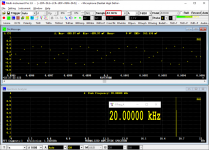
No Interpolation
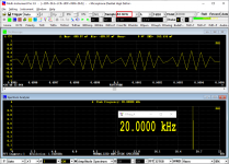
Linear Interpolation
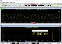
SINC Interpolation
By the way, AP has clearly states here that their CSD uses FFT (instead of DFT, thus power of 2 for FFT size) and zero padding. (Waterfall (CSD) Plots with APx - Audio Precision)
...you will have to connect these sparse N-point discrete spectral samples on the screen to make the spectrum look continuous. If you use straight lines, you are using linear interpolation between them.
You are right that this is how it's mostly done. However, it would be better to do a "stairs" plot, which would clearly show the frequency bins without connecting the dots by straight (or whatever) lines.
...AP has clearly states here that their CSD uses FFT (instead of DFT, thus power of 2 for FFT size) and...
FFT used to be limited to 2^n lengths. However, I believe there are FFT codes that will work with just about any length (the FFT functions in Matlab or GNU Octave work with arbitrary lengths). Otherwise it's always possible to do a "normal" Fourier transform, which does not come with any length constraints. Todays comuters will do this so fast that you will not know there is a difference between a FFT and a "normal" Fourier transform.
Does anyoine here use Virtins with the RTX6001? Do you need to load an RTX driver for that?
Jan
Jan
I have the 6001 with Virtins. Works very,very well. You need to select the 6001 ASIO ADC/DAC in the setup. Also you would need the native USB driver loaded.
I have the 6001 with Virtins. Works very,very well. You need to select the 6001 ASIO ADC/DAC in the setup. Also you would need the native USB driver loaded.
the RTX ASIO driver works best
And how/where is that?
Jan
OK got it. Installed the RTX drivers.
First measurement, external loop-back. All harmonics of 1kHz below -140dB ??
Jan
First measurement, external loop-back. All harmonics of 1kHz below -140dB ??
Jan
Well I'm not really sure that my measurement is valid. I'm still down the bottom of the learning curve!
Jan
Jan
- Home
- Group Buys
- GB for Virtins MI Pro for RTX6001 autoranging/autoscaling & for soundcard end users