Well, I finally got done with a preliminary evaluation of several SPICE models for the MJL3281A and MJL1302A to compare their simulated performance, mainly of ft vs collector current, with the data sheet values. This all started a while back when I was looking at the simulated performance of a power amplifier with a capacitive load of 2 uF in parallel with 8 Ohms using these devices for the output stage. I was trying to see if I could get the thing stable for this load with no output inductor. It turned out that the simulated open-loop output inductance of the amp was so large that a major resonance occurred at about 100 kHz, preventing stability from being achieved with any reasonable unity loop gain frequency with the capacitive load. In a previous thread involving Fred and myself (which I can't seem to locate at the moment), it became apparent that the models he was using with his simulator and the models I was using, provided by On Semiconductor, were quite different. We got very different results for the output inductance using the same test circuit.
This subject came up again in the thread about the amp in the Randy Slone book. But seeing that Randy Slone thread title keep coming up again and again made me feel like giving Randy a break - and the discussion of models really didn't have anything to do with the original thread topic anyway. So I thought I'd post the results of my evaluation in a new thread specifically about the SPICE models for these devices. My main purpose is to end up with a modified model whose simulated output inductance will be as close as possible to that of the real devices, assuming the real devices match up with the data sheet. Actually, I'd like as many of the parameters to match up as closely as possible with reality, but I'm starting with ft vs frequency. The desire to compare simulated and data sheet ft values came from the following site: http://www.reed-electronics.com/ednmag/archives/1996/042596/09df3.htm. There they have an expression for the output inductance of an emitter follower as follows:
Lout = R / (2 * pi * ft)
where R is the internal plus external base resistance. This clearly shows the need for accurate ft in the model to get accurate output inductance. I'll also look at the internal base resistance, but that will be the topic of another post to this thread. I have three models for each of the NPN and PNP devices: the On Semiconductor models, the PSpice models for the Toshiba 2SC3281 and 2SA1302, and the models Fred posted in the thread I referred to earlier. I'm not sure if Fred's models were for the Toshiba or On Semiconductor devices though.
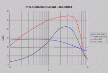
The simulation test circuits for ft are similar to those shown in http://www.diyaudio.com/forums/showthread.php?postid=235089#post235089, except that I put the DC supply in the base instead of the emitter (to keep a constant Vce) and set the collector supply to 10Vdc to match the value used in the ft vs Ic plots in the data sheets. I temporarily placed a current source in the emitter to set the currents to the desired values, then determined Vbe. Then I used these Vbe values to set the currents when doing the actual ft simulation. The result is a spreadsheet with two plots and the raw data. So without further ado, here is a plot for ft vs collector current for the MJL3281A.
This subject came up again in the thread about the amp in the Randy Slone book. But seeing that Randy Slone thread title keep coming up again and again made me feel like giving Randy a break - and the discussion of models really didn't have anything to do with the original thread topic anyway. So I thought I'd post the results of my evaluation in a new thread specifically about the SPICE models for these devices. My main purpose is to end up with a modified model whose simulated output inductance will be as close as possible to that of the real devices, assuming the real devices match up with the data sheet. Actually, I'd like as many of the parameters to match up as closely as possible with reality, but I'm starting with ft vs frequency. The desire to compare simulated and data sheet ft values came from the following site: http://www.reed-electronics.com/ednmag/archives/1996/042596/09df3.htm. There they have an expression for the output inductance of an emitter follower as follows:
Lout = R / (2 * pi * ft)
where R is the internal plus external base resistance. This clearly shows the need for accurate ft in the model to get accurate output inductance. I'll also look at the internal base resistance, but that will be the topic of another post to this thread. I have three models for each of the NPN and PNP devices: the On Semiconductor models, the PSpice models for the Toshiba 2SC3281 and 2SA1302, and the models Fred posted in the thread I referred to earlier. I'm not sure if Fred's models were for the Toshiba or On Semiconductor devices though.
The simulation test circuits for ft are similar to those shown in http://www.diyaudio.com/forums/showthread.php?postid=235089#post235089, except that I put the DC supply in the base instead of the emitter (to keep a constant Vce) and set the collector supply to 10Vdc to match the value used in the ft vs Ic plots in the data sheets. I temporarily placed a current source in the emitter to set the currents to the desired values, then determined Vbe. Then I used these Vbe values to set the currents when doing the actual ft simulation. The result is a spreadsheet with two plots and the raw data. So without further ado, here is a plot for ft vs collector current for the MJL3281A.
Attachments
This may be straying a bit.....
But some of you guys think that the ON versions are better than the Toshiba ones.
According to a buddy who was in that department when it was Motorola:
The very first ones that they sold were Toshibas that they bought, without any inking, and the "batwing" logo was put on by Motorola. Reason was that they could not get theirs right.
The ON parts are a second source. Second source implies that it is as close as possible, if not indeed identical, in every way that can be. Otherwise, new parts would have to go through an evaluation process at darn near any company that used lots of them. And that is not what a second source is supposed to be.
Jocko
More data
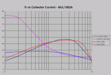
...and below is a plot for ft vs Ic of the MJL1302A. Clearly, the models for the MJL3281A are all pretty far off from reality, though the new On Semiconductor model for the MJL1302A looks at least reasonable. For small-signal analysis, the ft value for Ic of 100 mA is probably the most important. For the MJL3281A at 100 mA, the On Semiconductor model is more than a factor of six low for ft. So this says if the model can be tweaked to get this right, my previous estimates of power amp performance with a capacitive load will have been shown to be very pessimistic. This weekend I'm going to play around with the parameters of the On Semiconductor models in an attempt to get the plots to match up with the data sheets as closely as possible. I'll keep y'all posted on what happens. I'm going to try to fix the DC parameters first, then go for ft vs current. I'll also have a look at the internal base resistance if time allows.
...and below is a plot for ft vs Ic of the MJL1302A. Clearly, the models for the MJL3281A are all pretty far off from reality, though the new On Semiconductor model for the MJL1302A looks at least reasonable. For small-signal analysis, the ft value for Ic of 100 mA is probably the most important. For the MJL3281A at 100 mA, the On Semiconductor model is more than a factor of six low for ft. So this says if the model can be tweaked to get this right, my previous estimates of power amp performance with a capacitive load will have been shown to be very pessimistic. This weekend I'm going to play around with the parameters of the On Semiconductor models in an attempt to get the plots to match up with the data sheets as closely as possible. I'll keep y'all posted on what happens. I'm going to try to fix the DC parameters first, then go for ft vs current. I'll also have a look at the internal base resistance if time allows.
Attachments
Jocko,
Just to clarify, the curves marked as "data sheet" are from the On Semiconductor data sheet. All the other curves are simulated data. I didn't include the Toshiba data sheet info.
Just to clarify, the curves marked as "data sheet" are from the On Semiconductor data sheet. All the other curves are simulated data. I didn't include the Toshiba data sheet info.
Well, I don't know why all this ON-bashing, but to me the ON- models are way closer to the data sheet then any of the other ones. Since the data sheets are generated by actually characterizing the "average" device that is my reference.
The Pspice models clearly are a joke. Any decent text on semiconductor physics will show at least the general shape as shown by the ON-models.
Jan Didden
The Pspice models clearly are a joke. Any decent text on semiconductor physics will show at least the general shape as shown by the ON-models.
Jan Didden
Our resident simulation "expert" (Phred) has told me countless times that the PSpice models are dreck. If what is here is typical, perhaps he is right.
Yes, the ON model looks like what one would expect, even if the data sheet said elsewise.
As for ON in general, I suspect that they are as good now as the Toshibas. I just find it hard to believe that they are "way better", as some claim.
Jocko
Yes, the ON model looks like what one would expect, even if the data sheet said elsewise.
As for ON in general, I suspect that they are as good now as the Toshibas. I just find it hard to believe that they are "way better", as some claim.
Jocko
Re: More data
Great work Andy....cheers
andy_c said:Well, I finally got done with a preliminary evaluation of several SPICE models for the MJL3281A and MJL1302A to compare their simulated performance, mainly of ft vs collector current, with the data sheet values. This all started a while back when I was looking at the simulated performance of a power amplifier with a capacitive load of 2 uF in parallel with 8 Ohms using these devices for the output stage. I was trying to see if I could get the thing stable for this load with no output inductor. It turned out that the simulated open-loop output inductance of the amp was so large that a major resonance occurred at about 100 kHz, preventing stability from being achieved with any reasonable unity loop gain frequency with the capacitive load. In a previous thread involving Fred and myself (which I can't seem to locate at the moment), it became apparent that the models he was using with his simulator and the models I was using, provided by On Semiconductor, were quite different. We got very different results for the output inductance using the same test circuit.
This subject came up again in the thread about the amp in the Randy Slone book. But seeing that Randy Slone thread title keep coming up again and again made me feel like giving Randy a break - and the discussion of models really didn't have anything to do with the original thread topic anyway. So I thought I'd post the results of my evaluation in a new thread specifically about the SPICE models for these devices. My main purpose is to end up with a modified model whose simulated output inductance will be as close as possible to that of the real devices, assuming the real devices match up with the data sheet. Actually, I'd like as many of the parameters to match up as closely as possible with reality, but I'm starting with ft vs frequency. The desire to compare simulated and data sheet ft values came from the following site: http://www.reed-electronics.com/ednmag/archives/1996/042596/09df3.htm. There they have an expression for the output inductance of an emitter follower as follows:
Lout = R / (2 * pi * ft)
where R is the internal plus external base resistance. This clearly shows the need for accurate ft in the model to get accurate output inductance. I'll also look at the internal base resistance, but that will be the topic of another post to this thread. I have three models for each of the NPN and PNP devices: the On Semiconductor models, the PSpice models for the Toshiba 2SC3281 and 2SA1302, and the models Fred posted in the thread I referred to earlier. I'm not sure if Fred's models were for the Toshiba or On Semiconductor devices though.
The simulation test circuits for ft are similar to those shown in http://www.diyaudio.com/forums/showthread.php?postid=235089#post235089, except that I put the DC supply in the base instead of the emitter (to keep a constant Vce) and set the collector supply to 10Vdc to match the value used in the ft vs Ic plots in the data sheets. I temporarily placed a current source in the emitter to set the currents to the desired values, then determined Vbe. Then I used these Vbe values to set the currents when doing the actual ft simulation. The result is a spreadsheet with two plots and the raw data. So without further ado, here is a plot for ft vs collector current for the MJL3281A.
andy_c said:...and below is a plot for ft vs Ic of the MJL1302A. Clearly, the models for the MJL3281A are all pretty far off from reality, though the new On Semiconductor model for the MJL1302A looks at least reasonable. For small-signal analysis, the ft value for Ic of 100 mA is probably the most important. For the MJL3281A at 100 mA, the On Semiconductor model is more than a factor of six low for ft. So this says if the model can be tweaked to get this right, my previous estimates of power amp performance with a capacitive load will have been shown to be very pessimistic. This weekend I'm going to play around with the parameters of the On Semiconductor models in an attempt to get the plots to match up with the data sheets as closely as possible. I'll keep y'all posted on what happens. I'm going to try to fix the DC parameters first, then go for ft vs current. I'll also have a look at the internal base resistance if time allows.
Great work Andy....cheers
Jan:
>The Pspice models clearly are a joke.<
IME, many of them are. Spice is useful, but unless you are sure that your models are trustworthy (which is when?), better take the results with a large pinch of salt.
I have built circuits that appeared fine in the simulator, but proved pretty much impossible to get working in the real world
But I have also made circuits that performed far better than what the simulator predicted.
Jocko:
>Phred has told me countless times that the PSpice models are dreck. If what is here is typical, perhaps he is right.<
My experience suggests the same, time and time again.
But note that at least ft-Ic and capacitance-voltage curves can be found in many data sheets, so it is possible for hard workers like Andy C to plot the "simulated" curves against reality and locate the differences.
So what do you do when you are interested in Early voltages and other parameters that are _not_ stated in the data sheet?
Anyone know of an affordable but decent curve-tracer kit? 🙂
Nice post, Andy!
regards, jonathan carr
jcarr said:Jan:
>The Pspice models clearly are a joke.<
IME, many of them are. Spice is useful, but unless you are sure that your models are trustworthy (which is when?), better take the results with a large pinch of salt.
I have built circuits that appeared fine in the simulator, but proved pretty much impossible to get working in the real world
But I have also made circuits that performed far better than what the simulator predicted.
[snip]
nice post, Andy!
regards, jonathan carr
Jonathan,
I used to use a spreadsheet-based model maker from an early IsSpice version called, surprisingly, ModelMaker. Basically you put in as many parameters as you can find on the data sheet, guess on the once you are not sure about, and the program generates the model file. I need to see if I still have it.
But over the years I have gone back from trying to simulate everything until the last volt, amp or Hz. Nowadays I use the simulator more as a "proof of concept" tool and then built a prototype. I find that faster: you need a few iterations in the PCB layout anyway and this way you can combine that with electrical tweaking. (The big boys call it "concurrent engineering", I call it common sense).
Thanks to Andy, we are again reminded that the map is not the world!
Enjoy the weekend,
Jan Didden
Jan:
I've been looking at MultiSim 7, not the least because it has an optional model maker function. Looking at the device models included with a lot of EDA packages has led me to believe that a home-brewed model couldn't possibly be any worse.
Your description of ModelMaker from IsSpice suggests that it is a stand-alone program (or interfaces with another spreadsheet program like Excel?). Is there any place to download a copy, or purchase?
>Over the years I have gone back from trying to simulate everything until the last volt, amp or Hz. Nowadays I use the simulator more as a "proof of concept" tool and then built a prototype.<
Similar situation here. Getting bitten a lot at first is a good way to learn quickly.
>Thanks to Andy, we are again reminded that the map is not the world!<
Very true. And those were only the semiconductors. The board layout is also an issue for stability and performance, and at times the passive components can cause problems as well.
regards, jonathan carr
jcarr said:(...)So what do you do when you are interested in Early voltages and other parameters that are _not_ stated in the data sheet?(...)
Good point. I decided that I wanted to try getting as near to "data sheet clone" performance in my tweaked model as possible. So I started by trying to duplicate the so-called "Gummel plots" of ln(Ic) and ln(Ib) vs Vbe described in Massobrio and Antognetti. So I take plots of Ic vs Vbe and plots of beta vs Ic to reconstruct these. However, the Gummel plots must be done at Vcb = 0, and the data sheet plots are done with Vce = 20 V. So the first thing I need to do is "back out" the Early effect from the data to normalize it to Vcb = 0. So I need to know the Early voltage. As soon as I try to get it from the standard curve tracer plots, I see that they don't fit the theory of all intersecting at a point at all. Not even close. Then there's the reverse mode parameters like reverse Early voltage and so forth. That stuff isn't available from the data sheet at all.
This ended up being rather time consuming, so I decided to just tweak the AC parameters to try to get the ft vs Ic curves to match the data sheets as well as I can.
On a positive note, messing around with the formulas for Early effect modeling in Massobrio and Antognetti was really an eye-opener. I must admit that I previously had some confusion regarding the "down and dirty" specifics of the Early effect. But after pounding my head into the wall for a while on this, the light finally came on. I highly recommend this book to anyone interested in transistor modeling. It's really good.
Tweaked MJL3281A model
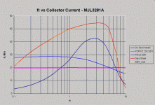
Here's an update of the model tweaking. I adjusted the CJE, TF, XTF and ITF parameters of the On Semiconductor MJL3281A model to get the ft vs Ic curve to be as close as possible to the data sheet. I wasn't able to emulate the very sharp dropoff of ft at high currents, so the best I could do was split the error. This makes the ft start dropping off at lower currents than the data sheet, yet the final ft value at the highest current is larger than the data sheet value. However, it's possible to get very good agreement with the data sheet in the low-current region by tweaking only CJE and TF. The final model is included below. I've also included a new plot of ft vs Ic that includes this modified model. The modified model is the yellow trace. Next step is to do a similar thing for the MJL1302A.
.MODEL Qmjl3281a_mod npn
+IS=6.5498e-11 BF=139.247 NF=1.00176 VAF=46.776
+IKF=10 ISE=7.75232e-12 NE=3.34341 BR=4.98985
+NR=1.09511 VAR=4.32026 IKR=4.37516 ISC=3.25e-13
+NC=3.96875 RB=11.988 IRB=0.111742 RBM=0.102914
+RE=0.00127227 RC=0.209833 XTB=0.115253 XTI=1.03146
+EG=1.11986 CJE=1.0531e-08 VJE=0.4 MJE=0.450375
+TF=2.6464e-9 XTF=1000 VTF=2.06045 ITF=175
+CJC=5e-10 VJC=0.4 MJC=0.85 XCJC=0.959922
+FC=0.1 CJS=0 VJS=0.75 MJS=0.5
+TR=1e-07 PTF=0 KF=0 AF=1
Attachments

I read this whole discussion with great interest, and I have found in the past that some simulations didn't make a whole lot of sense but I didn't suspect models.
Anyway, back to the topic. an actual device can have many different behaviors under difference circumstance. The model has just limited number of degrees of freedom so there is a compromise (in mimicing a complicated set of bahaviors from a limited number of variables).
so maybe the ft-current relationship is sacrificed in the process for other relationships deemed more important by On Semi?
BJT models
i do not remember when and what models I posted but would imagine I did.
Here are the ones that came with my Spice program. They are modeled with the AREA factor a have subcircuit to include the base spreading resistance I believe.
.SUBCKT QSC3281 1 2 3
* TERMINALS: C B E
* 200 Volt 15 Amp SiNPN Power Transistor 12-03-1991
Q1 1 2 3 QPWR .67
Q2 1 4 3 QPWR .33
RBS 2 4 9.5
.MODEL QPWR NPN (IS=1.63P NF=1 BF=150 VAF=254 IKF=12 ISE=1.34N NE=2
+ BR=4 NR=1 VAR=20 IKR=16.5 RE=22.1M RB=4 RBM=.4 IRB=5.556U RC=4.84M
+ CJE=481P VJE=.6 MJE=.3 CJC=312P VJC=.22 MJC=.2 TF=5.33N TR=204N)
+ XTB=1.5 PTF=120 XTF=1 ITF=9.6)
.ENDS
.SUBCKT QSA1302 1 2 3
* TERMINALS: C B E
* 200 Volt 15 Amp SiPNP Power Transistor 12-03-1991
Q1 1 2 3 QPWR .67
Q2 1 4 3 QPWR .33
RBS 2 4 9.5
.MODEL QPWR PNP (IS=1.63P NF=1 BF=130 VAF=254 IKF=11 ISE=1.34N NE=2
+ BR=4 NR=1 VAR=20 IKR=16.5 RE=12.1M RB=4 RBM=.4 IRB=5.556U RC=4.84M
+ CJE=1.09N VJE=.6 MJE=.3 CJC=708P VJC=.22 MJC=.2 TF=5.33N TR=204N)
+ XTB=1.5 PTF=120 XTF=1 ITF=9.6)
.ENDS
I have not examined them very closely to see how good the models are.
The genral form for a BJT model in Spice is:
QXXXXXXX NC NB NE <NS> MNAME <AREA> <OFF> <IC=VBE, VCE> <TEMP=T>
http://newton.ex.ac.uk/teaching/CDHW/Electronics2/userguide/sec3.html#3.4.3
Re: BJT models
That's an interesting way of doing the model. It looks like this double transistor approach has a similar effect to the XCJC parameter used to model the collector-base capacitance being distributed across the base spreading resistor. From Massobrio and Antognetti, "The capacitance XCJC*CJC is placed between the internal base node and the collector. (1 - XCJC)*CJC is the capacitance from external base to collector, while CJC is the total base-collector capacitance." So it looks like this is the equivalent of XCJC=0.33.
Looks like these are the same models you posted earlier as the data agrees with what I had. I previously missed the subcircuit usage though.
Originally posted by Fred Dieckmann Here are the ones that came with my Spice program. They are modeled with the AREA factor a have subcircuit to include the base spreading resistance I believe.
That's an interesting way of doing the model. It looks like this double transistor approach has a similar effect to the XCJC parameter used to model the collector-base capacitance being distributed across the base spreading resistor. From Massobrio and Antognetti, "The capacitance XCJC*CJC is placed between the internal base node and the collector. (1 - XCJC)*CJC is the capacitance from external base to collector, while CJC is the total base-collector capacitance." So it looks like this is the equivalent of XCJC=0.33.
Looks like these are the same models you posted earlier as the data agrees with what I had. I previously missed the subcircuit usage though.
"I previously missed the subcircuit usage though."
More likely I failed to include it. Thanks for you work of shedding light on transistor models. It should be very helpful to the "Spice Guys"
Fred
PS Do you do jfets...........
More likely I failed to include it. Thanks for you work of shedding light on transistor models. It should be very helpful to the "Spice Guys"
Fred
PS Do you do jfets...........
Originally posted by Fred Dieckmann (...)More likely I failed to include it.(...)
Looks like you included it and I missed it. 😉 Here's the original thread:
http://www.diyaudio.com/forums/showthread.php?postid=174227#post174227
As to the JFETs, I haven't gotten to that chapter yet. I suspect that eventually I'll try my hand at them.
Modified MJL1302A model
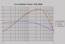
Here's the modified MJL1302A model as I mentioned I'd do. I used a similar approach to the MJL3281A model mods, adjusting CJE, TF and ITF to try to match the data sheet's ft vs Ic as closely as possible. As you can see, the original On Semiconductor models were already pretty close. The new model is the yellow trace and the data sheet values are the red trace. I got rid of the PSPICE model, as it was so bad that it messed up the graph scaling. This is really a minor tweak, but it may be of interest, especially to those trying to get the most accurate small-signal model possible.
.MODEL Qmjl1302a_mod pnp
+IS=3.25053e-12 BF=60.3363 NF=0.992063 VAF=19.8199
+IKF=7.18352 ISE=3.25712e-12 NE=3.42487 BR=5.15499
+NR=1.03617 VAR=2.77936 IKR=9.38159 ISC=2.5e-13
+NC=3.89405 RB=0.776136 IRB=0.0998107 RBM=0.776136
+RE=0.000613663 RC=0.0424163 XTB=1.43773 XTI=1
+EG=1.05 CJE=1.0690e-08 VJE=0.728073 MJE=0.42161
+TF=2.9458e-9e-09 XTF=1000 VTF=4.11586 ITF=380
+CJC=1.79861e-09 VJC=0.814822 MJC=0.473271 XCJC=1
+FC=0.8 CJS=0 VJS=0.75 MJS=0.5
+TR=1e-07 PTF=0 KF=0 AF=1
Attachments
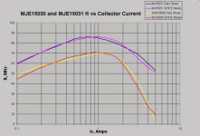
Here is some MJE15030/31 data
I had a look at the MJE15030 and MJE15031 models as well, with the thought that I'd have to tweak those too. It turns out that the ft vs Ic of these models agrees quite well with the data sheet curves of same.
One thing that I found interesting was the rolloff of ft at high currents for the NPN device is much more abrupt than for the PNP. The SPICE model tracks this sudden change quite well. But the model for the MJL3281A did not compare nearly as well to its data sheet rolloff of ft at high currents, despite my having made numerous attempts to tweak this. What's going on here?
Thinking about this question made me realize something I hadn't thought of previously. The parameter I was using to adjust the falloff of ft at high currents is called IKF. This interacts with another parameter, TF (the forward transit time). For a "semi-ideal" transistor, the ft increases with current at low currents, then becomes approximately constant at a certain current level, reaching a maximum value of 1/(2*pi*TF). Now the purpose of IKF is to make the forward transit time a function of current, rather than just being equal to TF. This then causes ft to drop off again at high currents. So in a nutshell, by tweaking IKF, one can adjust the rolloff of ft at high currents. But what does this really do? Well, it only adjusts the bandwidth of hFE. The rolloff of ft at high current is also influenced by the decrease of the low-frequency value of hFE at high currents (since ft is the product of the low-frequency hFE and the -3 dB bandwidth of hFE). This effect is dealt with strictly by the transistor DC parameters. So suppose the vendor didn't accurately model the falloff of DC beta at high currents. Guess what, the ft falloff at high currents will never be right either, no matter how you tweak IKF.
So I suspect that the inaccurate modeling of the falloff of ft at high currents for the MJL3281A is due to inaccurate modeling of the falloff of DC beta at high currents. But unfortunately I didn't check that. I assumed they couldn't possibly get the DC stuff wrong. Sigh.
At any rate, users of the On Semiconductor models for the MJE15030 and MJE15031 needing accurate modeling of ft vs Ic can be confident that the models predict this variation quite accurately out of the box.
Attachments
Andy, do you have a definition of the effect of the IKF parameter?
My semiconductor physics book is too old to include it, since it
was added in later Spice versions. Howver, the info i have
managed to find about it on the net and in various docs. does
not suggest that it models any frequency dependence. My
understanding is that its purpose is only to model high injection
(aka. beta drop), ie. the decrease in hfe at high values of Ic,
which AFAIK is not frequency dependent. It seems that IKF
is the value of Ic where hfe has dropped by 50%.
BTW, have you managed to model a beta drop that coincides
reasonably well with datasheets? What I mean here is a
hfe vs. Ic diagram. Although I haven't looked at the particular
BJTs you are considering, I have looked at a number of others.
None of the models came even close to the datasheets. I have
also DIY'ed Spice models for some transistors I couldn't find
models for, and there seems to be no way to get a beta drop
that is large enough to coincide with datasheets. IKF does not
have a strong enough effect, which is somewhat surprising
since I think it is intended to model the high injection equation.
Similarly, I also have not found any models or managed to
design any myself that model the saturation region of a BJT
well. Have you checked this for the BJTs you are considering?
This should matter, I think, for the crossover-distorsion
simulations discussed in another thread and which you (I think)
simulated.
- Status
- Not open for further replies.
- Home
- Amplifiers
- Solid State
- Evaluation results: MJL3281A/MJL1302A SPICE Models